Basics of statistical theory
With all the quantum-computing topics I lately hear, read, and talk about, I thought it’s high time to refresh some basics of statistical theory. Naturally, being a mathematical discipline, a great deal of formulas and equations are used to describe the nature of random outcomes. However, I prefer a more experimental approach where tests are executed and visualized with computer programs, which is why you’ll find Python code interlaced in this post. I encourage everybody reading this, to open a code editor, and play around with these programs.
The code snippets can mostly be run as is, except for a few helper functions in the utils.py script, which can be downloaded from the link at the end of this post.
Table of Contents
- Descriptive Statistics
- Data sampling
- Basic probabilistic rules
- Normal distribution
- Binomial distribution
- Large sample sizes
- Regression
- Confidence intervals
- Test of significance
- The Monte Carlo method
- The Bootstrap method
- Categorical data
- The Analysis of Variance (ANOVA) / F-Test
- Reproducibility and Replicability
- Summary of tests
- Resources
\( \newcommand\prob[1]{\mathrm{P}(#1)} \newcommand\cvec[1]{\begin{pmatrix}#1\end{pmatrix}} \newcommand\nullH[]{\mathrm{H_0}} \)
Descriptive Statistics
Descriptive statistics gives ways to summarize data with numbers and graphs. The importance of descriptive statistics lies in the communication of information.
There are several ways to communicate data, but the best format is graphical, that is as pictures. There are also several ways to visualize data, which usually depends on the nature of the data.
- pie charts or dot plots for qualitative data
- bar graph for quantitative data
- histograms are bar graphs, but allow for various bin widths
- height of the bar tells the number of subjects per horizontal scale
- percentages are given by \(\mathrm{area}=\mathrm{height}\times\mathrm{width}\).
- histograms are bar graphs, but allow for various bin widths
- Box-and-Whisker plot (or simply box plot) visualizes the data
using 5 key numbers:
- maximum, minimum, median, and first and third quartile (25th and 75th percentile) numbers.
- reduces the information of the data
- Scatter plot displays dots in data space
- useful to analyse relationships between different dimensions/properties of the data
The purpose of a statistical analysis is typically to compare the observed data to some kind of reference. Context is most important for statistical analyses and essential for graphical integrity.
Moreover, there are pitfalls when it comes to visualizing data, and too flashy graphics can sometimes obscure the information to be communicated.
Some notes on the following material: as a physicist, I sometimes might fall back into the “bad” habit (over this can be argued though) of using the standard error \(\mathrm{SE}\) and standard deviation \(\sigma\) and \(s\) interchangably, especially in the context of confidence intervals. This is an implicit application of descriptive statistics and should be understood as such.
import random
random.seed(42)

N = 300
x = [random.gauss(5, 2) for _ in range(N)]
bins = []
bin_edges = range(-1, 12)

xsrt = sorted(x)
idx = 0
for l, r in zip(bin_edges, bin_edges[1:]):
    while idx < N and xsrt[idx] < l:
        idx += 1
    lidx = idx
    while idx < N and xsrt[idx] < r:
        idx += 1
    ridx = idx
    bins.append([lidx, ridx])
for i, (lidx, ridx) in enumerate(bins):
    hbar = len(x[lidx:ridx])
    bar = "   " + "o"*hbar
    print(str(bin_edges[i]))
    print(bar)
print(bin_edges[-1])
-1
   o
0
   oooooo
1
   ooooooooo
2
   oooooooooooooooooooooooooooo
3
   ooooooooooooooooooooooooooooooooooooooo
4
   ooooooooooooooooooooooooooooooooooooooooooooooooooooooo
5
   ooooooooooooooooooooooooooooooooooooooooooooooooooooooooooooooooo
6
   oooooooooooooooooooooooooooooooooooooooooooooooooooo
7
   ooooooooooooooooooooo
8
   oooooooooooo
9
   oooooooooo
10

11
Numerical summary measures
Mean
The average or mean of the entire data. The mean of a population is often designated as \(\mu\), whereas the (arithmetic) mean of a sample is
\begin{equation}\label{eq:mean} \bar{x} = \frac{1}{n}\sum_{i=1}^{n}{x_i} \end{equation}
Expected value
In probability theory, the expected value of a random variable \(X\), denoted as \(E(X)\), is a generalization of the mean of all possible, independent realizations of \(X\). So,
\begin{equation}\label{eq:expected_value} E(X) = \sum_i{x_i\,p_i} \end{equation}
where the probabilities (weights) \(\sum_i{p_i} = 1\) and \(x_i\) are a finite number of outcomes. Moreover, for a random sample of \(n\) independent observations, the expected value of the sample mean \(E(\bar{x}) = \mu\).
If \(X\) follows a (continuous) probability distribution \(\prob{x}\), then the mean of the distribution (also called first moment) is
\begin{equation}\label{eq:mean_continuous} \mu = \int_{-\infty}^{\infty}{x\,\prob{x}\,\mathrm{d}x} \end{equation}
Median
The number that is larger than half the data and smaller than the other half. (When the data distribution is symmetric, the mean and median are the same.)
For skewed data it is often better to use the median to avoid biasing from outliers, or unimportant data groupings.
import random
random.seed(42)
from utils import list_fmt

N = 12
x = [random.random() for _ in range(N)]
xsrt = sorted(x)
if N % 2 == 0:
    median = 0.5*(xsrt[N//2 - 1] + xsrt[N//2])
else:
    median = xsrt[N//2]
mean = sum(x)/len(x)

print("Sorted data")
print(list_fmt(':6d', N).format(*range(N)))
print(list_fmt(':6.4f', N).format(*xsrt))
print(f"Median = {median:.4f}")
print(f"Mean = {mean:.4f}")
Sorted data
[      0      1      2      3      4      5      6      7      8      9     10     11 ]
[ 0.0250 0.0298 0.0869 0.2186 0.2232 0.2750 0.4219 0.5054 0.6394 0.6767 0.7365 0.8922 ]
Median = 0.3485
Mean = 0.3942
n-th percentile
The n-th percentile is a score below which a given percentage of scores in its frequency distribution falls. For example, the 50th percentile is the median.
Standard deviation
The standard deviation is a measure of the amount of variation or dispersion of a set of data values. A low standard deviation indicates that the values tend to be close to the mean of a dataset, while a high standard deviation indicates that the values are spread out over a wider range.
Since the expected value of a random variable \(E(X)\) is \(\mu\), the standard deviation of \(X\) is
\begin{align}\label{eq:std}
\sigma &= \sqrt{E[(X-\mu)^2]} = \sqrt{E(X^2) - E(X)^2}
&= \sqrt{\sum_{i=1}^{n}{p_i(x_i - \mu)^2}}
\end{align}
If the random variable follows a probability distribution \(\prob{x}\), the standard deviation is
\begin{equation}\label{eq:std_continuous} \sigma = \sqrt{\int_{-\infty}^{\infty}{(x-\mu)^2\prob{x}\,\mathrm{d}x}} \end{equation}
Note, that the standard deviation of a sample (of independent measurements) is usually designated
\begin{equation}\label{eq:std_sample} s = \sqrt{\frac{1}{n}\sum_{i=1}^{n}{(x_i - \bar{x})^2}} \end{equation}
In some cases, the standard deviation of a sample is used to estimate the population variance, by applying Bessel’s correction. It uses \(n−1\) instead of \(n\) in the formula for the sample variance and sample standard deviation, where \(n\) is the number of observations in a sample. This method corrects the bias in the estimation of the population variance.
import random
random.seed(42)
from utils import list_fmt

def sqrt_newton(a, max_iters=30, tol=1e-12):
    a0 = a
    for _ in range(max_iters):
        a_prev = a
        a = a - 0.5*(a*a-a0)/a
        if abs(a_prev - a) < tol:
            return a

N = 12
x = [random.random() for _ in range(N)]
mu = sum(x)/len(x)
squares = [(xi-mu)**2 for xi in x]
sigma = sqrt_newton(sum(squares)/len(squares))

print("Sorted data")
print(list_fmt(':6.4f', N).format(*sorted(x)))
print(f"Sigma = {sigma:6.4f}")
Sorted data
[ 0.0250 0.0298 0.0869 0.2186 0.2232 0.2750 0.4219 0.5054 0.6394 0.6767 0.7365 0.8922 ]
Sigma = 0.2822
Variance
Variance is the expectation of the squared deviation of a random variable \(X\) from its mean \(\mu\). It is a measure of dispersion, meaning it is a measure of how far a set of numbers is spread out from their average value.
\begin{equation}\label{eq:variance} \mathrm{Var}(X) = E[(X-\mu)^2] = \sigma^2 \end{equation}
It’s the second central moment of the probability distribution of a random variable.
Skewness
Skewness is the third central moment of a probability distribution of a random variable. It measures the asymmetry of the distribution.
\begin{equation}\label{eq:skewness} \mu_3 = E[(X-\mu)^3] = \int_{-\infty}^{\infty}{(x-\mu)^3\prob{x}\,\mathrm{d}x} \end{equation}
Kurtosis
Kurtosis is the fourth central moment of a probability distribution of a random variable. It measures the “peakyness” of the distribution.
\begin{equation}\label{eq:kurtosis} \mu_4 = E[(X-\mu)^4] = \int_{-\infty}^{\infty}{(x-\mu)^4\prob{x}\,\mathrm{d}x} \end{equation}
Distribution functions
A probability density function (PDF) gives the probability density \(f_X\) for a random variable \(X\) such that
\begin{equation}\label{eq:pdf} \prob{a \leq X \leq b} = \int_a^b{f_X(x)\,\mathrm{d}x} \end{equation}
Hence, the cumulative distribution function (CDF) of \(X\) is
\begin{equation}\label{eq:cdf} F_X(x) = \int_{-\infty}^x{f_X(u)\,\mathrm{d}u} \end{equation}
which follows \(\lim\limits_{x\to-\infty}{F_X}(x) = 0\) and \(\lim\limits_{x\to\infty}{F_X}(x) = 1\).
Data sampling
Statistical inference is used to estimate a parameter for a population by estimating the parameter on subsamples of the population.
Key terms used above
- Population: The entire group of subjects holding information of interest.
- Parameter: The quantity of interest about the population.
- Hyperparameter: In machine learning hyperparameters are tuneable parameters for a model’s learning/training process.
- Sample: a subset of data about the population obtained through, e.g. measurements or observations.
- Estimate/Statistic: the quantity of interest as measured in the sample
- Statistical inference: the process of estimating a parameter for a population by estimating the parameter on samples of the population.
Random sampling
Simple random sampling
All subjects from a population have an equal probability of being drawn with no further consideration.
Hereby, sampling can happend “with replacement”, meaning the subject is copied from the population and can be selected again in a later draw with the same probability, or “without replacement” when the population is taken from the population, thereby changing probabilities of subsequent draws.
Systematic random sampling / Interval sampling
Systematic sampling (also known as interval sampling) relies on arranging the population according to some ordering scheme and then selecting elements at regular intervals through that ordered list.
Stratified random sampling
When the population can be organized into homogeneous categories, so-called strata, stratified sampling might be useful. Thereby, each stratum is individually random-sampled, according to their relative sizes (sampling fractions).
Statistical vs Systematic error
Note that an estimate from a random sample is different from the true parameter, which is called the chance error, or statistical error. The bigger the sample size, the smaller the chance error. Moreover, the chance error can be computed, whereas the bias (systematic error) cannot.
\begin{equation}\label{eq:parameter_estimate} \mathrm{estimate} = \mathrm{parameter} + \mathrm{bias} + \mathrm{chance\ error} \end{equation}
Biases
A sample of convenience will introduce a bias to the statistic. A bias is a favouring of a certain outcome, which can have various kinds
- Selection bias involves individuals being more likely to be selected for study than others due to external influences.
- Confirmation bias involves the tendency to collect, select, or interpret the data such that it yields an expected result.
- Non-response bias is a phenomenon in which the results of surveys become non-representative because the participants disproportionately possess certain traits which affect the outcome.
- Voluntary response bias occurs when sample members are self-selected volunteers. This creates an overrepresentation of subjects with strong or extreme opinions in the sample.
Observation vs. Experiment
Observational studies can easily be misunderstood. They measure outcomes of interest and this can be used to establish association, but not causation. There may be confounding factors that are associated with such studies.
For causation, an experiment is required: a test is assigned to subjects in the test group (randomly sampled), but not to subjects in the control group. If possible, the control group is treated with a placebo, a neural test. This assures that both groups are equally affected by the placebo effect: the idea of being tested may have an effect itself. The outcomes are compared afterwards. The experiment should be double-blind: neither the subjects nor the evaluators know the assignment to test and control.
Randomization assures that influences other than the test operate equally on both groups, apart from differences due to chance, and it allows to assess the chance effects by comparing the outcomes in the two groups.
Interpretation of probability
The probability of an event is defined as the proportion of times this event occurs in many repetitions. For example, in a coin toss we write
\begin{equation}\label{eq:P_coin_toss} \prob{\mathrm{heads}} = 50.0\% \end{equation}
The long-run interpretation of probability can make it difficult to interpret it for single events. In some contexts, people use probability in another interpretation, as subjective probability, which is not based on experiments, and could be estimated differently by different people.
Basic probabilistic rules
Complement rule
Probabilities are always between 0 and 1. Let’s assume, we have an event A, then
\begin{equation}\label{eq:complement_rule} \prob{\lnot A} = 1 - \prob{A} \end{equation}
Equally likely outcomes
If event A has a \(n\) different outcomes which are equally likely, then
\begin{equation}\label{eq:equal_probability_rule} \prob{A} = \frac{\mathrm{number\ of\ outcomes\ in\ A}}{n} \end{equation}
Addition rule
If event A is mutually exclusive with an event B, i.e. cannot occur at the same time, then
\begin{equation}\label{eq:addition_rule} \prob{A \mathrm{\ or\ } B} = \prob{A} + \prob{B} \end{equation}
Multiplication rule
If two events A, B are independent, i.e. if knowing that A occurs does not change the probability that B occurs, then
\begin{equation}\label{eq:multiplication_rule} \prob{A \mathrm{\ and\ } B} = \prob{A} \cdot \prob{B} \end{equation}
-
Example
With these four rules, we are already able to solve many problems. For instance, let’s roll a die three times. What is \(\prob{\mathrm{at\ least\ one\ }6}\)?
\begin{align} \mathrm{at\ least\ one\ }6 \mbox{ (in 3 rolls)} \quad=\quad \mbox{6 at 1st roll} \quad\mbox{or}\quad \mbox{6 at 2nd roll} \quad\mbox{or}\quad \mbox{6 at 3rd roll} \end{align}
These events are unfortunately not mutually exclusive, so the addition rule doesn’t help. Let’s use the complement rule instead: \(\begin{align} \mathrm{P}(\mathrm{at\ least\ one\ }6) &= 1 - \prob{\lnot 6} \\ &= 1 - \prob{\lnot 6 \mbox{ at 1st roll} \quad\mbox{and}\quad \lnot 6 \mbox{ at 2nd roll} \quad\mbox{and}\quad \lnot 6 \mbox{ at 3rd roll}} \\ &= 1 - \prob{\lnot 6 \mbox{ at 1st roll}} \cdot \prob{\lnot 6 \mbox{ at 2nd roll}} \cdot \prob{\lnot 6 \mbox{ at 3rd roll}} \\ &= 1 - \frac56\cdot\frac56\cdot\frac56 \\ &= 1 - \frac{125}{216} \approx 0.4213 \sim 42.13\% \end{align}\)
Conditional probability
A conditional probability of B given A is
\begin{equation}\label{eq:cond_prob} \prob{B | A} = \frac{\prob{A\mbox{ and }B}}{\prob{A}} \end{equation}
This can be rearranged into a general multiplication rule:
\begin{equation}\label{eq:general_multiplication_rule} \prob{A\mbox{ and }B} = \prob{A}\cdot\prob{B | A} \end{equation}
This is useful for computing probabilities by total enumeration.
-
Example
For instance, if it is known that \(\prob{\mbox{spam}}=20\%\), \(\prob{\mbox{money | spam}}=8\%\), and \(\prob{\mbox{money | ham}}=1\%\), what is the probability that ‘money’ appears in an e-mail? In order to answer this question, we can artifically introduce the event ‘spam/ham’. The event ‘money appears in the e-mail’ can be written as:
\begin{align} \mbox{money appears and e-mail is spam}\quad\mbox{or}\quad\mbox{money appears and e-mail is ham} \end{align}
These events are mutually exclusive and therefore we can use the addition rule: \(\begin{align} \prob{\mbox{money}} &= \prob{\mbox{money and spam}} + \prob{\mbox{money and ham}}\\ &= \prob{\mbox{spam}}\cdot\prob{\mbox{money | spam}} + \prob{\mbox{ham}}\cdot\prob{\mbox{money | ham}}\\ &= 20\%\cdot 8\% + 80\%\cdot 1\% = 0.2\cdot 0.08 + 0.8\cdot 0.01 = 0.024 = 2.4\% \end{align}\)
Baye’s rule
Through Eqs. (\ref{eq:cond_prob}) & (\ref{eq:general_multiplication_rule}), we can derive Baye’s theorem:
\begin{equation}\label{eq:bayes_theorem} \prob{B | A} = \frac{\prob{A\mbox{ and }B}}{\prob{A}} = \frac{\prob{B\mbox{ and }A}}{\prob{A}} = \frac{\prob{B}\cdot\prob{A | B}}{\prob{A}} \end{equation}
In some cases, \(\prob{A}\) can be computed. Then the Baye’s theorem can be written as
\begin{equation}\label{bayes_theorem_expanded} \prob{B | A} = \frac{\prob{B}\cdot\prob{A | B}}{\prob{A}} = \frac{\prob{B}\cdot\prob{A | B}}{\prob{B}\cdot\prob{A | B} + \prob{\lnot B}\cdot\prob{A | \lnot B}} \end{equation}
The Baye’s theorem takes a previously known probability \(\prob{B}\), known as the prior probability, and updates it according to the Baye’s rule to arrive at the posterior probability \(\prob{B | A}\). \(\prob{A}\) is often referred to as marginal probability, and \(\prob{A | B}\) as the likelihood.
-
Example
Suppose that 1% of the population has a certain disease \(D\), and there’s a test for the presence of the disease. If an infected person is tested, then there’s a 95% chance that the test is positive (\(+\)), but if the person is not infected, then there’s still a 2% chance that a test gives an erroneous positive result. That’s called a false positive.
Given that a person tests positive, what are now the chances that the person has the disease?
Let’s first define what we know:
\[\begin{align} \prob{D} = 1\% \quad\Rightarrow\quad \prob{\lnot D} = 99\% \\ \prob{+ | D} = 95\% \quad\mbox{and}\quad \prob{+ | \lnot D} = 2\% \\ \end{align}\]Therefore, we can use Baye’s theorem to calculate
\[\begin{align} \prob{D | +} &= \frac{\prob{D}\ \prob{+ | D}}{\prob{+}} \\ &= \frac{\prob{D}\ \prob{+ | D}}{\prob{+ | D}\ \prob{D} + \prob{+ | \lnot D}\ \prob{\lnot D}} \\ &= \frac{0.01 \cdot 0.95}{0.95\cdot 0.01 + 0.02\cdot 0.99} \approx 32.42\% \end{align}\] -
Warner’s randomized response model
What percentage of students have cheated during an exam in college? The problem here is that most students may be too embarrassed to answer truthfully in a survey.
Here, randomization may help out. First, instruct students to toss a coin twice. If the student get’s ‘tails’ on the first toss, he/she should answer Q1, otherwise Q2:
- Q1) Have you ever cheated on an exam in college?
- Q2) Did you get ‘tails’ on the second toss?
The answer we are going to get will be partly random. A ‘yes’ could be due to the student answering Q1 and having cheated on an exam, or it could be due to the student answering Q2 in getting tails on the second toss. The key point here is that we cannot really tell what an individual ‘yes’ means, but by looking at all the answers collectively, we can actually estimate the proportion of cheaters.
\[\begin{align} \prob{\mbox{yes}} &= \prob{\mbox{yes and Q1}} + \prob{\mbox{yes and Q2}}\\ &= \prob{\mbox{yes | Q1}}\ \prob{\mbox{Q1}} + \prob{\mbox{yes | Q2}}\ \prob{\mbox{Q2}} \end{align}\]
\[\begin{align} \prob{\mbox{yes | Q1}} &= \frac{\prob{\mbox{yes}} - \prob{\mbox{yes | Q2}}\ \prob{\mbox{Q2}}}{\prob{\mbox{Q1}}}\\ &\approx \frac{\prob{\mbox{yes}} - 0.5\cdot 0.5}{0.5}\\ \end{align}\]Solving for the probability of interest \(\prob{\mbox{yes Q1}}\), we get Now, we only have to estimate from data what \(\prob{\mbox{yes}}\) is. Say, we have 27 ‘yes’ and 30 ‘no’ answers. This means \(\prob{\mbox{yes}} = 27 / (27+30) \approx 47\%\), and we get \(\prob{\mbox{yes | Q1}} \approx 44\%\).
-
Exercise 1
A multiple choice exam has 10 questions. Each question has 3 possible answers, of which one is correct. A student knows the correct answers to 4 questions and guesses the answers to the other 6 questions.
It turns out that the student answered the first question correctly. What are the chances that the student was merely guessing?
\[\begin{align} \prob{G | +} &= \frac{\prob{G \mbox{ and } +}}{\prob{+}} = \frac{\prob{+ | G}\ \prob{G}}{\prob{+}} \\ &= \frac{\prob{+ | G}\ \prob{G}}{\prob{+ | G}\ \prob{G} + \prob{+ | \lnot G}\ \prob{\lnot G}} \\ &= \frac{(\frac13)(\frac{6}{10})}{(\frac13)(\frac{6}{10}) + (1)(\frac{4}{10})} \end{align}\] -
Exercise 2
There are three boxes on the table: The first box contains 2 quarters, the second box contains 2 nickels, and the last box contains 1 quarter and 1 nickel. You choose a box at random, then you pick a coin at random from the chosen box.
If the coin you picked is a quarter, what’s the chance that the other coin in the box is also a quarter?
With “qq” for “quarter-quater box”, “qn” for “quarter-nickel” box, and “q” for “picked a quarter”:
\[\begin{align} \prob{qq | q} &= \frac{\prob{q|qq}\ \prob{qq}}{\prob{q}} \\ &= \frac{\prob{q|qq}\ \prob{qq}}{\prob{q | qq}\ \prob{qq} + \prob{q | qn}\ \prob{qn} + \prob{q | nn} \prob{nn}} \\ &= \frac{\prob{q|qq}\ \prob{qq}}{\prob{q | qq}\ \prob{qq} + \prob{q | qn}\ \prob{qn}} \\ &= \frac{(\frac11)(\frac13)}{(\frac11)(\frac13) + (\frac12)(\frac13)} \end{align}\]
Normal distribution
Histograms often look bell-shaped, i.e. follow the normal curve. If this is the case, as a rule of thumb 2/3 of the data fall within 1 standard deviation of the mean, which is called the empirical rule. 95% of the data lie within 2 standard deviations from the mean, and 99.8% within 3 standard deviations.
The normal distribution is determined by two parameters, the mean \(\bar{x}\) and the standard deviation \(s\). To compute areas under the normal curve (called normal approximation), data \(x\) first has to be standardized
\begin{equation}\label{eq:standardize} z = \frac{x - \bar{x}}{s} \end{equation}
\(z\) is often called standardized value or z-score. It measures the deviation from the mean in units of standard deviations. Consequently, the z-score has a mean of 0 and a standard deviation of 1.
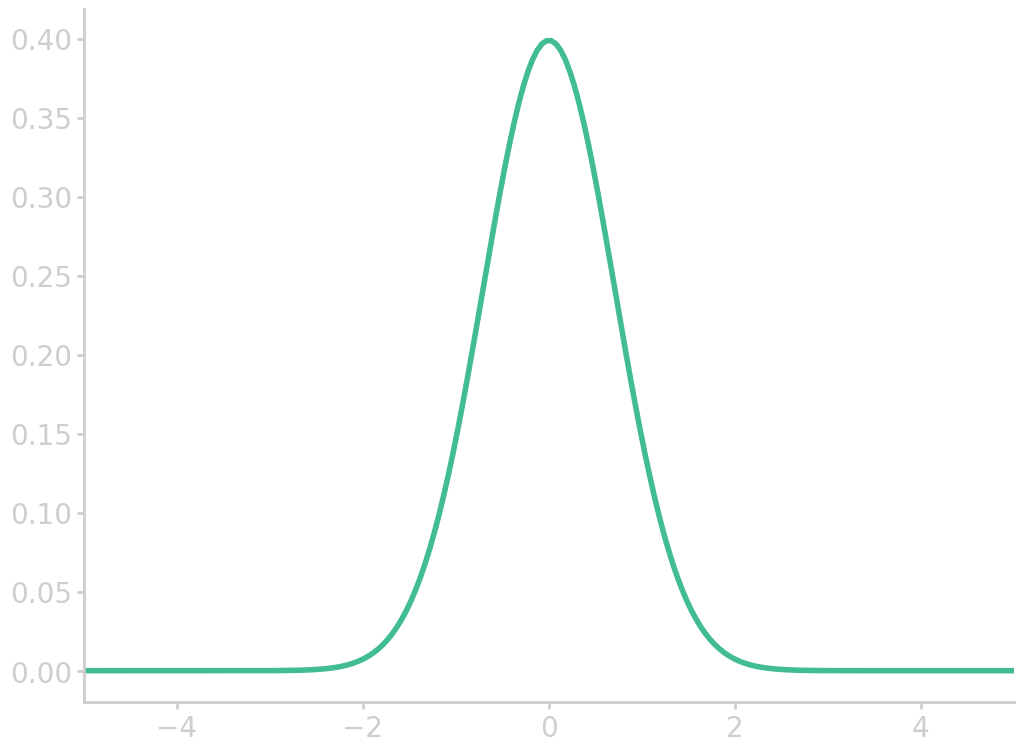
The normal distribution is described by
\begin{equation}\label{eq:normal_dist} f(x) = \frac{1}{\sqrt{2\pi}} \exp{\left(-\frac{z(x)^2}{2}\right)} \end{equation}
import numpy as np
import matplotlib.pyplot as plt

z = np.linspace(-5, 5, 200)
fz = np.exp(-z*z)/np.sqrt(2*np.pi)
plt.plot(z, fz)
plt.xlim(-5, 5)

filename = 'images/norm_dist.png'
plt.savefig(filename)
plt.close()
return filename
Binomial distribution
A binomial setting is an independently repeated event where outcomes can be ‘success’ or ‘failure’.
For instance, the possibility that 2 out of 5 newborns are girls comes from a binomial setting, and can be computed by the total enumeration of all possibilities. However, such problems can quickly grow large and become hard to count. The binomial coefficient counts the number of ways one can arrange k successes in n experiments
\begin{equation}\label{eq:binomial_coeff} \cvec{n \ k} = \frac{n!}{k!(n-k)!} \end{equation}
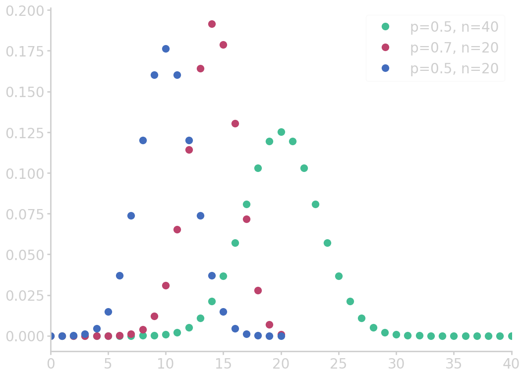
The binomial probability function is given by
\begin{equation}\label{eq:binomial_func} \prob{\mbox{k successes in n experiments}} = \cvec{n \ k} p^{k}(1-p)^{n-k} \end{equation}
from numpy import asarray
from utils import comb
import matplotlib.pyplot as plt

for p, n in zip([0.5, 0.7, 0.5], [40, 20, 20]):
    k = asarray(range(0, n+1))
    binom_c = asarray([comb(n, i) for i in k])
    binomial = binom_c * p**k * (1-p)**(n-k)
    plt.plot(k, binomial, marker='o', ms=10, lw=0,
             label=f'p={p}, n={n}')
plt.xlim(0, 40)
plt.legend()

filename = 'images/binomial_dist.png'
plt.savefig(filename)
plt.close()
return filename
Random variables
Outcomes of experiments are due to chance. We can define the number of successes as \(X\) which is called a random variable. If we calculate the probability of a certain number of successes, say \(\prob{X=2}\), with the binomial distribution, we say \(X\) has the binomial distribution.
Such functionals can be visualized with probability histograms, a theoretical construct, which illustrates the probabilities of a certain number of experiments depending on the number of successes.
Normal approximation to the binomial
As the number of experiments gets larger, the probability histogram of the binomial distribution looks similar to the normal curve. In fact, we can approximate binomial probabilities using normal approximation: for standardization, we subtract \(n\cdot p\) and divide by \(\sqrt{np(1-p)}\).
Remember that a simple random sample selects subjects without replacement. This is not a binomial setting, because \(p\) changes after a subject has been removed. If the population is big enough though, sampling with or without replacement is almost the same, and thus the number of successes will have approximately the binomial distribution.
-
Example
For example, let’s say we want to calculate the chance of winning at most 12 prices in 50 games, where the chance of winning a price is \(1/5\).
We know that the probability distribution roughly looks like a normal distribution, with a mean of 10. So,
\begin{align} z = \frac{12-np}{\sqrt{np(1-p)}} = \frac{12-10}{\sqrt{8}} \approx 0.71 \end{align}
Numerically integrating the normal distribution up to a z-score of 0.71 will give the answer, roughly 76.11%.
\begin{equation}\label{eq:error_function} \Phi(z) = \frac12 + \frac12\mathrm{erf}\left(\frac{z}{\sqrt{2}}\right) \end{equation}
Large sample sizes
The mean of a population is often designated with \(\mu\) and its standard deviation \(\sigma\).
The expected value of a random draw is the average \(\mu\), as it is for \(n\) draws. The expected value of the sample average \(\mathrm{E}(\bar{x}_n)\), is also the average \(\mu\). The standard error describes how far off the expected value is from the population average
\begin{equation}\label{eq:expected_value_2} \mathrm{E}(\bar{x}_n) = \mu \end{equation}
The square root law is key for statistical inference
\begin{equation}\label{eq:sqrt_law} \mathrm{SE}(\bar{x}_x) = \frac{\sigma}{\sqrt{n}} \end{equation}
It shows that the standard error becomes smaller if we use a larger sample size \(n\), and does not depend on the size of the population.
The expected value and standard error for a sum of a sample \(S_n\) is therefore given by
\begin{equation} \mathrm{E}(S_n) = n\mu\quad\quad\quad\mathrm{SE}(S_n) = \sqrt{n}\sigma \end{equation}
This is useful in the case where we might want to count the number of votes for an election forecasting model (we can simply label the votes 1 or 0 and sum up the sample for the total number of expected votes).
For simulated data drawn from a probability distribution, the expected value and standard error is the same. If the random variable \(X\) that is simulated has \(k\) possible outcomes \(x_1, \ldots, x_k\), then
\begin{equation} \mu = \sum_i^k{x_i}\prob{X=x_i}\quad\quad\quad\sigma^2 = \sum_i^k{(x_i-\mu)^2}\prob{X=x_i} \end{equation}
If the random variable \(X\) has a probability density \(f\), such as when \(X\) follows the normal distribution, then
\begin{equation} \mu = \int_{-\infty}^{\infty} xf_X(x)\mathrm{d}x\quad\quad\quad\sigma^2 = \int_{-\infty}^{\infty} (x-\mu)^2f_X(x)\mathrm{d}x \end{equation}
-
Example: Coin toss
Toss a coin 100 times. How many ‘tails’ do you expect to see? Give or take how many?
Let’s say ‘tails’ is 1 and ‘heads’ is 0. We know that \(\prob{0} = \prob{1} = 1/2\). The number of tails can be from 0 to 100, however the expected value is \(\mathrm{E}(S_n) = 100\cdot\mu\) = 50, where the average of the sum of draws can be calculated by summing up all possible outcomes weighted by their probabilities \(\mu = 0\cdot\prob{0} + 1\cdot\prob{1} = 1/2\). The standard error is therefore around \(\mathrm{SE}(S_n) = \sqrt{100}\sigma = 5\), where the standard deviation is \(\sigma^2=(0-\frac12)^2 \frac12 + (1-\frac12)^2 \frac12 = \frac14\).
import mt19937 as Random
Random.MT_seed(64)
for _ in range(10):
    coin_tosses = [int(Random.bernoulli(0.5)) for _ in range(100)]
    print(sum(coin_tosses), end='  ')
49 49 42 60 41 42 43 50 52 52
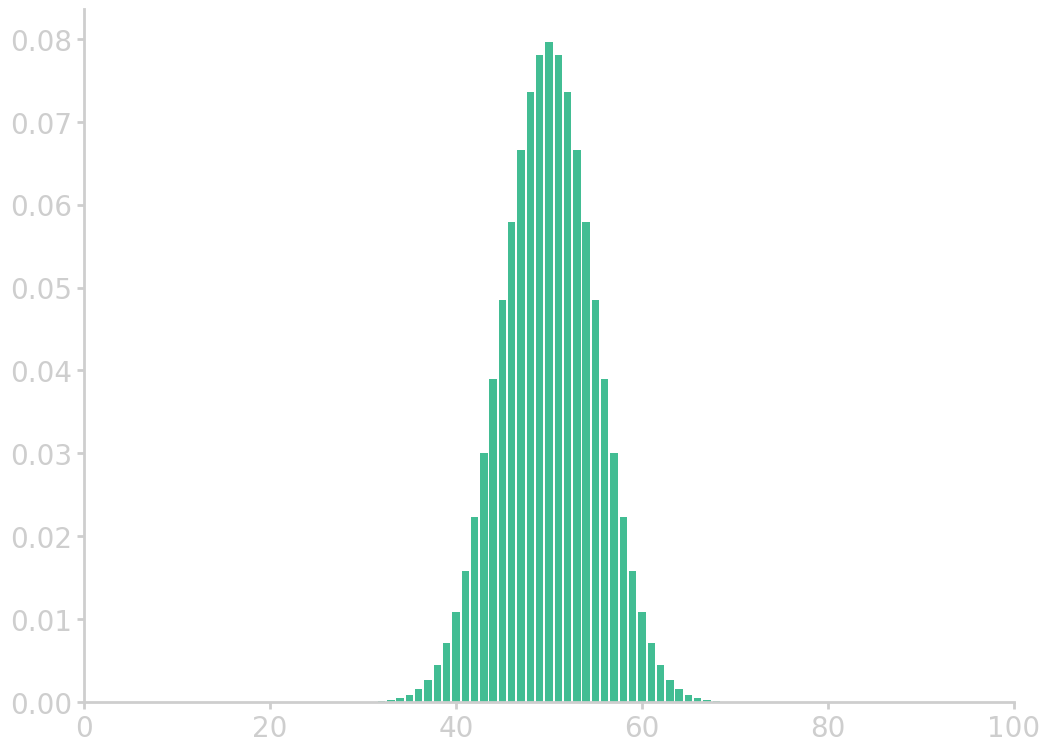
In principle, sum statistics from 0 all the way to 100 are possible. The probabilities for these outcomes are given by the binomial distribution.
from numpy import asarray
from utils import comb
import matplotlib.pyplot as plt

p = 0.5
n = 100
k = asarray(range(0, n+1))
binom_c = asarray([comb(n, i) for i in k])
binomial = binom_c * p**k * (1-p)**(n-k)
plt.bar(k, binomial)
plt.xlim(0, 100)

filename = 'images/cointoss_dist.png'
plt.savefig(filename)
plt.close()
return filename
Law of large numbers
In the square root law Eq. (\ref{eq:sqrt_law}), we saw that when the sample size increases, the standard error of the mean \(\mathrm{SE}(\bar{x}_n)\) approaches zero. This is known as the law of large numbers. It applies to averages (not to sums) when sampled with replacement.
The Central Limit Theorem
In the section Binomial distributions, we saw that when \(n\) is large enough, the distribution resembles a normal distribution. This is an example of the Central Limit Theorem: It says that when we sample with replacement and \(n\) is large, then the sampling distribution of the sample average (or of the sum), approximately follows the normal curve.
This is the probably most important theorem in statistical theory.
The key point of the theorem is that we know that the sampling distribution of the statistic is normal no matter what the population distribtion is. That is, if we sample \(n\) times from any distribution with mean \(\mu\) and standard deviation \(\sigma\), then we yield a normal distribution centered at \(\mathrm{E}(\bar{x}_n)=\mu\) and with a spread of \(\mathrm{SE}(\bar{x}_n)=\frac{\sigma}{\sqrt{n}}\).
The conditions where the central limit theorem applies are
- sampling with replacement, or simulation of independent random variables from the same distribution
- statistic of interest is a sum (averages are actually also sums, but weighted)
- sample size is large enough: the more skewed the population distribution is, the larger the required sample size \(n\).
Regression
Prediction is a key task of statistics. Regression is a very simple, and versatile technique which accomplishes just that. Before regression can be discussed a few basics have to be covered.
Correlation
Relationships between two quantitative variables can have various forms. One could increase, when the other increases, or exactly the opposite. The functional nature of the variables can also show various behaviours, e.g. it could be that one increases exponentially, while the other increases linearly.
The strength of a linear association is measured by the correlation coefficient. The data are \((x_i, y_i)\) for \(i=1, \ldots, n\),
\begin{equation}\label{eq:correlation_coeff} r = \frac{1}{n}\sum_{i=1}^n{\frac{x_i - \bar{x}}{s_x}\cdot\frac{y_i - \bar{y}}{s_y}} \end{equation}
where the correlation coefficient is the sum of products of the standardized data in \(x\) and \(y\), and always between \(-1\) and \(1\).
Therefore pairs of data can be numerically summarized by the corresponding pairs of mean and standard deviation, and the correlation coefficient. As a convention, we call the variable on the horizontal axis predictor, and the variable on the vertical axis response.
Remember that correlation does not mean causation.
Least squares method
If the relationship is linear, we can use \(\hat{y_i} = a + bx_i\) to approximate the data \(y_i\). The least squares technique tries to find \(a, b\) which minimize the sum of squared distances between the data \(y_i\) and \(\hat{y_i}\).
That is, for \(n\) pairs \((x_1, y_1), \ldots, (x_n, y_n)\), find \(a, b\) which minimize
\begin{equation}\label{eq:lsqrs} \sum_{i=1}^{n}{(y_i - \hat{y_i})^2} = \sum_{i=1}^{n}{(y_i - (a + bx_i))^2} \end{equation}
where \(\hat{y_{}}\) is called the regression line. It turns out that the linear parameters \(a\) and \(b\) can be found using calculus, i.e. \(b=r\frac{s_y}{s_x}\) and \(a=\bar{y}-b\bar{x}\).
Another interpretation of the regression line is that it predicts the average of \(y\), when given \(x\).
Regression to the mean
Regression to the mean is a phenomenon which has to be considered in the design of experiments. It has various definitions, but in essence it arises when a sample point of a random variable is extreme (almost outlier), a future point is likely to be closer to the mean or average.
It is best explained by an example:
Take a hypothetical example of 1000 subjects of similar age who were examined and scored on the risk of a heart attack. The group of 50 people with the greatest risk (almost outliers) were used to measure the effect of an intervention (such as a healthier lifestyle). Even if the interventions are worthless, the group would show an improvement on the next examination, because of regression to the mean. This can lead to wrong conclusions about interventions and is called the regression fallacy.
Predictions from regression
Note that when predicting \(x\) from \(y\), we need to compute the regression line anew.
For any linear regression, the scatter of the data is ideally football-shaped. Then, we may use the normal approximation for the \(y\) values given \(x\), i.e. all points near \(x\) are approximately normally distributed around the mean. This means, to standardize we subtract off the predicted value \(\hat{y_{}}\) and divide by \(\sqrt{1-r^2}\cdot s_y\).
Residuals
Differences between predicted \(\hat{y_{}}\) values and the data \(y\) are called residuals, and are a good indicator how well the fitted curve describes the data. Residuals should be unstructured, close to zero.
Residuals can identify many problems of regression:
-
If the residuals indicate that the data does not behave linearly, we can try transformations such as squaring, square-root, or logarithm, in order to linearize the data, fit it, and then use the inverse transformation to yield our predictions.
-
A residual plot can also be used to identify a heteroscedastic (fan-shaped) scatter of the data, in which case certain transformations might allieviate the problem.
-
Another problem of regression is the handling of outliers. Outliers can be hinting to interesting causes or phenomena, or be simply typos in the data. Either way, they should be examined. Outliers with high leverage, influence the regression line heavily, and thus are called influential points.
-
Moreover, extrapolation of the regression line should be avoided, as a linear relationship may often break outside a certain range.
Regression analyses often report an R-squared value, which is the squared correlation coefficient \(R^2 = r^2\). The interpretation is that it gives the fraction of the variation in \(y\) that is explained by the regression line, because \(1-r^2\) is the fraction of variation in \(y\) left over in the residuals.
Confidence intervals
Sampling from a population results in a statistic which is off due to chance error, and the standard (or statistical) error tell us by how much.
We can use confidence intervals to give a precise statement how likely it is for a statistic of a random variable to fall within a certain range. According to the central limit theorem, the sample statistic will be normally distributed and according to the empirical rule, there is a 68% chance that the sample average will be no more than 1\(\sigma\) away from the population average, 95% chance for 2\(\sigma\), and so on.
So, we can give confidence intervals like
\begin{equation}\label{eq:confidence_intervals} \mathrm{estimate} \pm z\cdot\mathrm{SE} \end{equation}
where the width of the confidence interval is often called margin of error.
The probabilities are determined by the z-score, that is \(\mathrm{erf}\left(z/\sqrt{2}\right)\):
| z-score | probability |
|---|---|
| (in %) | |
| 1 | 68.2689 |
| 2 | 95.4499 |
| 3 | 99.7300 |
| 4 | 99.9937 |
| 5 | 99.9999 |
| 0.67 | 50 |
| 1.15 | 75 |
| 1.96 | 95 |
This also means a confidence interval tells us how likely it is for the population’s \(\mu\) to fall in a certain range. Unfortunately, we often cannot know the population’s \(\sigma\). However, the bootstrapping principle (more details later) states that we can estimate \(\sigma\) by its sample version and still get an approximately correct confidence interval.
Test of significance
Assume, we toss a coin and get 7 tails. Can we conclude that the coin is unfair?
The null hypothesis, denoted \(\nullH\), is the default hypothesis which usually claims that a quantity to be measured is zero, or in other words that there is no difference between two situations or characteristics of a population.
\begin{equation} \nullH:\quad \prob{T} = \frac12 \end{equation}
The alternative hypothesis, \(\mathrm{H_A}\), states that there is a different chance process that generates the data
\begin{equation} \mathrm{H_A}:\quad \prob{T} \neq \frac12 \end{equation}
Hypothesis testing proceeds by collecting and evaluating whether the data is compatible with \(\nullH\) or not, in which case \(\nullH\) is rejected. In hypothesis testing, it is often the case that the logic is indirect, i.e. one assumes the null hypothesis and tries to reject the assumption.
The z-test
The test statistic measures how far off the data is from the assumption that \(\nullH\) is true
\begin{equation}\label{eq:hypothesis_z_statistic} z = \frac{\mathrm{observed} - \mathrm{expected}}{\mathrm{SE}} \end{equation}
where \(\mathrm{observed}\) is the statistic that is appropriate for assessing \(\nullH\), and \(\mathrm{expected}\) and \(\mathrm{SE}\) are the expected value and the standard error of the statistic, computed under the assumption that \(\nullH\) is true. Large absolute values of \(z\) are evidence against \(\nullH\), the larger \(|z|\) the stronger the evidence.
The strength of the evidence is measured by the p-value, or observed significance level. The p-value is the probability of getting a value of \(z\) as extreme or more extreme than the observed \(z\), assuming \(\nullH\) is true (it measures the evidence against \(\nullH\)). But if \(\nullH\) is true, then \(z\) follows a normal distribution according to the central limit theorem, so the p-value can be computed with the normal approximation.
Note that the p-value does not give the probability that \(\nullH\) is true, as \(\nullH\) is either true or false, there are no chances involved.
Typically, a hypothesis is rejected if the p-value is smaller than 5%, which corresponds to a 2\(\sigma\) confidence width.
In physics however, only a \(5\sigma\) confidence is acceptable, which corresponds to roughly a 0.0001% p-value threshold.
\begin{equation}\label{eq:p_value} \mathrm{p} = c\cdot\mathrm{erfc}\left(\frac{|z|}{\sqrt{2}}\right) \end{equation}
where \(c\) is the coverage factor of the alternative hypothesis, usually \(\frac12\) or 1 if one-sided or two-sided.
-
Example
Let’s do an experiment to see whether Coke and Pepsi are distinguishable by taste alone. In the experiment 10 cups are filled at random with either Coke or Pepsi. A volunteer tastes all and correctly identified 7 of them.
\(\nullH\) represents the case where the volunteer cannot distinguish between Coke and Pepsi. So,
\[\begin{align} \nullH:&\quad\prob{0} = \prob{1} = \frac12 \\ \mathrm{H_A}:&\quad\prob{1} > \frac12 \end{align}\]This is a one-sided test: the alternative hypothesis for \(\prob{1}\) we are interested in is on one side of \(\frac12\). A two-sided alternative might be
\begin{align} \mathrm{H_A}:\quad\prob{1} \neq \frac12 \end{align}
In the one-sided test, the p-value will only be half as large. The z-score is
\begin{align} z = \frac{\mbox{observed sum} - \mbox{expected sum}}{\mbox{SE of sum}} = \frac{7 - 5}{1.58} = 1.27 \end{align}
where the \(\mathrm{SE} = \sqrt{np(1-p)} = \sqrt{10}\sqrt{\frac12\cdot\frac12}\) assumes \(\nullH\) is true.
This gives a p-value of
\[\begin{align} \mathrm{p} = \frac12\mathrm{erfc}\left(\frac{|z|}{\sqrt{2}}\right) = \frac12\mathrm{erfc}\left(\frac{1.27}{\sqrt{2}}\right) \approx 0.1020 \end{align}\]since 10.2% is larger than 5%, the hypothesis is typically not rejected.
Note that it is important to decide before testing whether a one-sided or two-sided test should be used, as changes during or after the experiment are not good.
The t-test
Say, we analyse drinking water on its lead concentration. The health guideline prescribes a concentration of no more than 15 ppb (parts per billion). Our measurements of five independent samples averages 15.6 ppb. Our measurement average could however be over the limit due to measurement error.
So,
\[\begin{align} \nullH:&\quad \mu = 15\,\mathrm{ppb}\\ \mathrm{H_A}:&\quad \mu > 15\,\mathrm{ppb} \end{align}\]We can try a z-test, but discover that for \(\mathrm{SE}\) unfortunately the standard deviation is unknown.
The t-test can be used if the standard deviation \(\sigma\) in an experiment is unknown or incompatible. We could estimate \(\sigma\) from the sample standard deviation \(s\), but for small sample sizes (about \(n\leq20\)) the normal approximation is not accurate enough.
In this case, the Student’s t-distribution with n-1 degrees of freedom
\begin{equation}\label{eq:student_t_distribution} f_n(t) = \frac{\Gamma\left(\frac{n+1}{2}\right)}{\sqrt{n\pi}\,\Gamma\left(\frac{n}{2}\right)}\left(1+\frac{t^2}{n}\right)^{-\frac{n+1}{2}} \end{equation}
import numpy as np
from math import gamma
import matplotlib.pyplot as plt

def student_t(x, n):
    N = (n + 1) / 2
    factor = gamma(N) / gamma(N-0.5) / np.sqrt(n*np.pi)
    return factor * (1+x**2/n)**(-N)

z = np.linspace(-5, 5, 200)
for n in [1, 2, 5, 10][::-1]:
    fz = student_t(z, n)
    plt.plot(z, fz, label=f"n = {n}")
plt.xlim(-5, 5)
plt.legend()

filename = 'images/t_dist.png'
plt.savefig(filename)
plt.close()
return filename
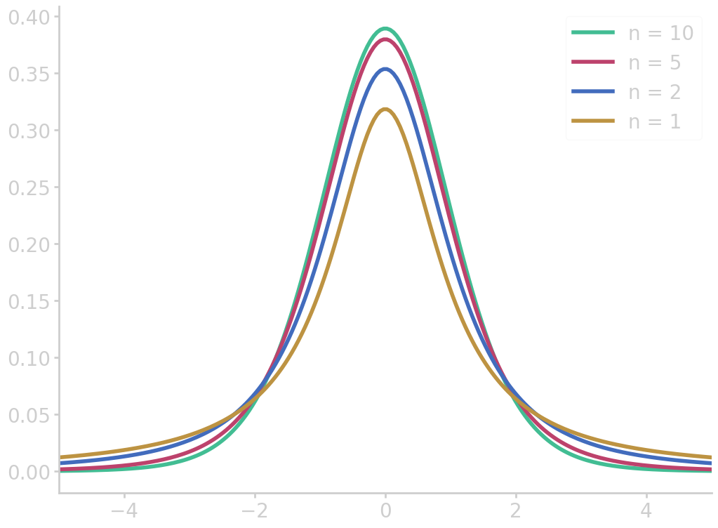
This distribution is slightly lower around the mean and have more area under the tails. The longer tails account for the additional uncertainty introduced by estimating \(\sigma\) by
\begin{equation} s = \sqrt{\frac{1}{n-1}\sum_{i=1}^{n}{(x_i-\bar{x})^2}} \end{equation}
The confidence interval should then be replaced by
\begin{equation} \bar{x} \pm t_{n-1}\mathrm{SE} \end{equation}
where the t-value is
\begin{equation}\label{eq:t_value} t_{n-1} = \frac{\bar{x} - \mu}{s\,/ \sqrt{n}} \end{equation}
Two-sample z-test
Say, we analyse polling rates for an election of the last and this month. The results of last month’s 1000 polls were \(p_{1}=55\%\) approval, and this month \(p_{2}=58\%\) approval from 1500 polls.
Now, we want to assess whether the proportions of likely voters are equal. It is common to look at the difference instead: \(p_{2}-p_{1}=0\).
The null hypothesis therefore is
\[\begin{align} \nullH:&\quad p_2 - p_1 = 0\\ \mathrm{H_A}:&\quad p_2 - p_1 \neq 0 \end{align}\]The central limit theorem applies to the difference just as it does to the statistics alone.
An important fact is that if \(p_1\) and \(p_2\) are independent, then the standard error of an addition or difference of individual standard errors is
\begin{equation}\label{eq:standard_error_addition} \mathrm{SE}(p_2-p_1) = \sqrt{\mathrm{SE}(p_1)^2 + \mathrm{SE}(p_2)^2} \end{equation}
So,
\begin{equation} z = \frac{(p_2 - p_1) - 0}{\sqrt{\sqrt{\frac{p_1(1-p_1)}{1000}}^2+\sqrt{\frac{p_2(1-p_2)}{1500}}^2}} = \frac{0.03}{0.0202} = 1.48 \end{equation}
This corresponds to a p-value of 13.89%.
Pooled estimates
We could have also pooled the samples, i.e. 1420 approvals out of 2500, so \(p_1=p_2=56.8\%\). The standard error then is
\begin{equation} \mathrm{SE}(p_2-p_1) = \sqrt{\frac{0.568(1-0.568)}{1500} + \frac{0.568(1-0.568)}{1000}} = 0.0202 \end{equation}
which essentially gives the same answer as before.
If one has reason to assume that \(\sigma_1=\sigma_2\), then one may use the pooled estimate
\begin{equation} s^2_{\mathrm{pooled}} = \frac{(n_1-1)\,s^2_1+(n_2-1)\,s^2_2}{n_1+n_2-2} \end{equation}
where \(n_1\) and \(n_2\) are the individual sample sizes. The pooled t-test is usually avoided though, because assuming that both standard deviations are equal is often problematic.
Paired-difference test
Say, we want to know whether husbands thend to be older than their wives. You gather data from five couples:
| husband's age | wife's age | age difference \(d_{i}\) |
|---|---|---|
| 43 | 41 | 2 |
| 71 | 70 | 1 |
| 32 | 31 | 1 |
| 68 | 66 | 2 |
| 27 | 26 | 1 |
The two-sample t-test is unfortunately not applicable since the two samples are not independent. Even if they were independent, the small differences in ages would not be significant since the standard deviations are larger for husbands and also for the wives. In other words, the two-sample z-test compares the differences to the fluctuations within each population. And in this case, the differences are small compared to the fluctuations within each population and therefore the two-sample z-test will not be applicable.
Since we have paired data, we can simply analyse the differences obtained from each pair with a regular t-test, which in this context of matched pairs is called paired t-test.
\[\begin{align} \nullH:\quad \mu &= 0 \quad\mbox{(population difference is zero)} \\ \bar{d} &= 7/5 = 1.4 \quad\mbox{and}\quad n=5 \\ \sigma_d &= s_d = \sqrt{\frac{2(2-1.4)^2}{n-1} + \frac{3(1-1.4)^2}{n-1}} \approx 0.5477 \\ \mathrm{SE}(\bar{d}) &= \frac{\sigma_d}{\sqrt{n}} \approx \frac{0.5477}{\sqrt{5}} \approx 0.2449 \\ t =& \frac{\bar{d}-\mu}{\mathrm{SE}(\bar{d})} = \frac{1.4 - 0}{0.5477 / \sqrt{5}} \approx 5.7155 \end{align}\]Reading off the p-values from a t-table, gives 0.4%, i.e. strong evidence for rejecting the null hypothesis.
If we didn’t know the age difference but only whether the husband was older or younger, we could use binary labels and the z-test
\begin{align} z = \frac{S_n-\frac{n}{2}}{\mathrm{SE}(S_n)} = \frac{5-\frac52}{\sqrt{5\frac12}} \approx 2.24 \end{align}
The p-value 2.5% of this sign-test is less significant than that of the paired t-test. This is because the latter uses more information, namely the size of the differences. On the other hand, the sign test has the virtue of easy interpretation due to the analogy to coin tossing.
Notes on testing
- statistically significant does not mean that the effect size is
important
- it is often helpful to complement a test with a confidence interval
- there is a general connection between confidence interval
- a confidence interval of 95% corresponds to a confidence width of 2\(\sigma\) and a p-value threshold of 5%
- there are two ways a test can result in a wrong decision:
- \(\nullH\) is true, but was erroneously rejected, a false positive: \(\prob{\mbox{false positive, type I error}} \leq 5\%\)
- \(\nullH\) is false, but there was failure to reject the null hypothesis (false negative, type II error)
- usually two-sample tests require that two samples are independent, or in special situations where the samples are dependent, e.g. to compare the treatment effect when subjects are randomized into treatment and control groups.
The Monte Carlo method
What if we are interested in an estimator \(\hat{\theta}\) for some parameter \(\theta\) and the normal distribution is not valid for the estimator? Or what if there is no formula for \(\mathrm{SE}(\hat{\theta})\)?
In such situations, simulations can often be used to estimate these quantities quite well. In fact, simulations may result in better estimates even in cases where the normal approximation is applicable!
We estimate a parameter \(\theta\) with an estimator \(\hat{\theta}\) which is based on a sample of \(n\) observations \(X_1, \ldots, X_n\) drawn at random from the population
\begin{equation} \hat{\theta} = \frac1n\sum_{i=1}^{n} X_i \end{equation}
The Monte Carlo method or simulation enables us to get an estimate for a parameter by the average of independent random variables that have expected value \(\theta\) through repeated sampling. The advantage of this approach is that the approximation error can be made arbitrarily small by increasing the sample size according to the law of large numbers.
Monte Carlo methods are a broad class of computational algorithms that rely on repeated random sampling to obtain numerical results, they are mainly used in optimization, numerical integration, and generating draws from a probability distribution.
The standard error of a statistic can also be determined using a Monte Carlo approach
\begin{equation}\label{eq:standard_error} \mathrm{SE}(\hat{\theta}) = \sqrt{\mathrm{E}(\hat{\theta} - \mathrm{E}(\hat{\theta}))^2} \end{equation}
which is the square root of the variance. Then, we can determine the standard error by
- getting N stamples of n observations, e.g. \(N=1000\) and \(n=100\)
- computing \(\hat{\theta}\) for each sample: \(\hat{\theta_1}, \ldots, \hat{\theta_N}\)
- computing the standard deviation of these N estimates:
\(s(\hat{\theta_1}, \ldots, \hat{\theta_N}) = \sqrt{\frac{1}{N-1}\sum_{i=1}^{N}{(\hat{\theta_i} - \bar{\hat{\theta}})^2}}\)
- Note that this is not an average of independent random variables. But it can be shown that the law of large numbers still applies: \(s(\hat{\theta_1}, \ldots, \hat{\theta_N}) \approx \mathrm{SE}(\hat{\theta})\)
This method is simply an application of the law of large numbers and relies on repeated resampling.
The Bootstrap method
The bootstrap method enables sampling even if we cannot draw as many samples as we wish, perhaps due to the fact that the sampling is too time consuming or expensive.
The plug-in principle allows us to calculate the mean of a population by calculating the mean of the sample instead.
The bootstrap uses the plug-in principle and a Monte Carlo method to approximate quantities such as \(\mathrm{SE}(\hat{\theta})\). The resoning behind the bootstrap is relatively simple
- we draw a sample \(X_1, \ldots, X_n\)
- since we cannot draw more samples, we apply the plug-in principle and use \(X_1, \ldots, X_n\) in place of the population
- we then simulate \(N\) bootstrap samples by drawing \(n\) times with
replacement from \(X_1, \ldots, X_n\) resulting in \(N\) estimates
- \(X^{\ast 1}_1, \ldots, X^{\ast 1}_n \quad\rightarrow\quad \hat{\theta^\ast_1}\)
- \(\vdots\)
- \(X^{\ast N}_1, \ldots, X^{\ast N}_n \quad\rightarrow\quad \hat{\theta^\ast_N}\)
- use \(\hat{\theta^\ast_1}, \ldots, \hat{\theta^\ast_N}\) to estimate the quantity of interest
The nonparametric bootstrap simulates bootstrap samples \(X^\ast_1, \ldots, X^\ast_n\) by drawing with replacement from a sample \(X_1, \ldots, X_n\). Sometimes, a parametric model is appropriate for the data, in which case we can use the parametric bootstrap method to simulate bootstrap samples from the model (e.g. a normal distribution), rather than a sample.
If there is dependence in the data (e.g. time series), then this needs to be incorporated, with the block bootstrap.
Bootstrap confidence intervals
If a sampling distribution of \(\hat{\theta}\) is approximately normal, then
\begin{equation} \left[\hat{\theta} - z_{\alpha/2}\mathrm{SE}(\hat{\theta}),\ \hat{\theta} + z_{\alpha/2}\mathrm{SE}(\hat{\theta})\right] \end{equation}
is an approximate (\(1-\alpha\))-confidence interval for \(\theta\), where we can use bootstrap to estimate \(\mathrm{SE}(\hat{\theta})\).
If \(\hat{\theta}\) is far from normal, then we use bootstrap to estimate the whole sampling distribution of \(\hat{\theta}\), not just \(\mathrm{SE}(\hat{\theta})\). This gives a bootstrap percentile interval
\begin{equation} \left[\hat{\theta}^{\ast}_{(\alpha/2)},\ \hat{\theta}^{\ast}_{(1-\alpha/2)}\right] \end{equation}
where \(\hat{\theta^{\ast}}_{(\alpha/2)}\) is the (\(\alpha/2\))-percentile of the approximated sampling distribution \(\hat{\theta^\ast_1}, \ldots, \hat{\theta^\ast_N}\).
If the approach needs to be less sensitive on the parameter \(\theta\), then we approximate the sampling distribution by bootstrapping \(\hat{\theta} - \theta\). This produces a more accurate confidence interval, the bootstrap pivotal interval
\begin{equation} \left[ 2\hat{\theta} - \hat{\theta}^{\ast}_{(1-\alpha / 2)},\ 2\hat{\theta} - \hat{\theta}^{\ast}_{(\alpha/2)} \right] \end{equation}
Bootstrapping for regression
We have data \((X_1, Y_1), \ldots, (X_n, Y_n)\) from a simple linear regression model
\begin{equation} Y_i = a + bX_i + e_i \end{equation}
where \(e_i\) are the error terms. From the data we can compute estimates \(\hat{\alpha},\ \hat{b}\). We can use bootstrap to get standard errors and confidence intervals in the following way:
- compute the residuals as estimates for the error terms \(\hat{e}_i = Y_i - \hat{a} - \hat{b}X_i\)
- resample from these residuals \(e^\ast_1, \ldots, e^\ast_n\)
- compute the bootstrapped responses \(Y^\ast_i = \hat{a} + \hat{b}X_i + e^\ast_i\)
This gives a bootstrap sample \((X_1, Y^\ast_1), \ldots, (X_n, Y^\ast_n)\) from which we can get the estimate \(\hat{a}^\ast\) and \(\hat{b}^\ast\) in the usual way. This can be repeated arbitrarily until yield the estimates for the parameters.
Categorical data
In 1912 the Titanic sank and over 1500 of the 2229 people on board died. Did the chances of survival depend on the ticket class?
| First | Second | Third | Crew | |
|---|---|---|---|---|
| Survived | 202 | 118 | 178 | 215 |
| Died | 123 | 167 | 528 | 698 |
This is an example of categorical data in form of a contingency table (also called crosstab). Such a type of table displays the multivariate frequency distribution of variables in a matrix format, i.e. it shows counts of categories.
Testing goodness-of-fit
In 2008 the producer of M&Ms stopped publishing their color distribution. Latest published percentages are
| Blue | Orange | Green | Yellow | Red | Brown |
|---|---|---|---|---|---|
| 24% | 20% | 16% | 14% | 13% | 13% |
Opening a bag of M&Ms, yields following counts
| Blue | Orange | Green | Yellow | Red | Brown |
|---|---|---|---|---|---|
| 85 | 79 | 56 | 64 | 58 | 68 |
Now the question is, are these counts consistent with the last published percentages?
The published percentages provide a “model” for which we can do a test of goodness-of-fit for the six categories. The null hypothesis \(\nullH\) corresponds to the scenario in which the color distribution data are given by the model. The alternative hypothesis is that the data are different from the model.
| Blue | Orange | Green | Yellow | Red | Brown | |
|---|---|---|---|---|---|---|
| observed | 85 | 79 | 56 | 64 | 58 | 68 |
| \(\nullH\) | 98.4 | 82 | 65.6 | 57.4 | 53.3 | 53.3 |
import numpy as np
import pandas as pd
from matplotlib import pyplot as plt

# read table above
df = pd.DataFrame(mnm_table).iloc[:, 2:].drop(1).reset_index(drop=True)
# set table names and clean up dataframe
df.columns = list(df.iloc[0])
df = df.drop(0).reset_index(drop=True)

# calculate chi2
chi2 = pd.DataFrame((df.iloc[0] - df.iloc[1])**2 / df.iloc[1]).T
chi2_sum = chi2.iloc[0].sum()
chi2_red = chi2_sum / (len(chi2.columns)-1)

# plot chi2 statistic
plt.bar(df.columns, chi2.iloc[0], alpha=0.8, label=r'$\chi^2_i$')
plt.axhline(chi2_red, ls='--', c='#bd426c', label=r'$\chi^2_\nu$')
plt.legend()
filename = 'images/m&m_chi2dist.png'
plt.savefig(filename)
plt.close()

print("chi2           = {:6.4f}".format(chi2_sum))
print("chi2 (reduced) = {:6.4f}".format(chi2_red))
chi2           = 8.5670
chi2 (reduced) = 1.7134
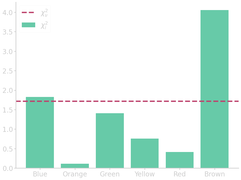
We combine the differences between the observed \(d_{\mathrm{obs}}\) and expected \(d_{\nullH}\) counts across all categories, to calculate the chi-square statistic
\begin{equation}\label{eq:chi2} \chi^2 = \sum{\frac{(d_{\mathrm{obs}} - d_{\nullH})^2}{\sigma^2}} \end{equation}
Often, the model variance \(\sigma^2\) is not known, but can be estimated with \(\sqrt{d_{\nullH}^2}\), so
\begin{equation} \chi^2 = \sum{\frac{(d_{\mathrm{obs}} - d_{\nullH})^2}{d_{\nullH}}} \end{equation}
For the M&M table, chi-square statistic is
\begin{align} \chi^2 = \frac{(85-98.4)^2}{98.4} + \frac{(79-82)^2}{82} + \cdots + \frac{(68-53.3)^2}{53.3} = 8.57 \end{align}
Large values of \(\chi^2\) are evidence against \(\nullH\), and a sign that the model is a poor match to the data. The \(\chi^2\) statistic depends on the degrees of freedom \(\nu = n - m\), where \(n\) is the number of observations and \(m\) the number of fitted parameters, here \(\nu\) is the number of categories \(-1\). So, to generalize the results we introduce the reduced chi square statistic
\begin{equation}\label{eq:chi2_reduced} \chi^2_\nu = \frac{\chi^2}{\nu} \end{equation}
As a rule of thumb, if the model variance is known, then \(\chi^2_\nu \gg 1\) indicates a poor model fit, or that the model has not fully captured the data. A value of \(\chi^2_\nu \sim 1\) means that the extent of the match between observations and estimates is in accord with the error variance. \(\chi^2_\nu \ll 1\) likely means that the model is overfitting the data, that is either the model is improperly fitting noise, or the error variance has been overestimated.
The p-value can be obtained by comparing the \(\chi^2\) value of the statistic to the \(\chi^{2}\) distribution \(\prob{\chi^2}\). It is the distribution of a sum of the squares of \(k\) independent standard normal random variables
from math import gamma
import numpy as np
import matplotlib.pyplot as plt

def chi2_dist(x, k):
    k2 = k/2
    factor = 2**k2 * gamma(k2)
    pdf = 1./factor * x**(k2-1) * np.exp(-0.5*x)
    return pdf

x = np.linspace(0, 10, 200)
for k in [1, 2, 3, 5, 8]:
    fx = chi2_dist(x, k)
    plt.plot(x, fx, label=f'k = {k}')
plt.xlim(0, 10)
plt.ylim(0, 1)
plt.ylabel('$\mathrm{P}(\chi^2)$', rotation=0)
plt.xlabel('$\chi^2$')
plt.legend()

filename = 'images/chi2_dist.png'
plt.savefig(filename)
plt.close()
return filename
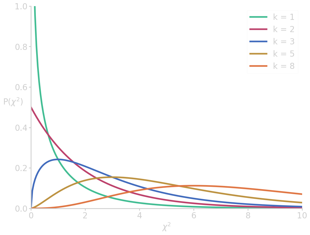
The cumulative distribution of \(\prob{\chi^2}\) measures how likely it is to measure a non-extreme value of \(\chi^2\), and thus the 1-p value. In this case, the p-value is computed to
from scipy.special import gammainc
import numpy as np
import matplotlib.pyplot as plt

x = np.linspace(0, 10, 200)
for k in [1, 2, 3, 5, 8]:
    cx = 1-gammainc(k/2, x/2)
    plt.plot(x, cx, label=f'k = {k}')
plt.xlim(0, 10)
plt.ylim(0, 1.02)
plt.ylabel('p-value', rotation=0)
plt.xlabel('$\chi^2$')
plt.legend()

filename = 'images/p_vs_chi2.png'
plt.savefig(filename)
plt.close()

p_val_mnm = 100*(1-gammainc(5/2, 8.57/2))
print("p-value (M&M 5 color distribution) = {:6.4f} %".format(p_val_mnm))
p-value (M&M 5 color distribution) = 12.7494 %
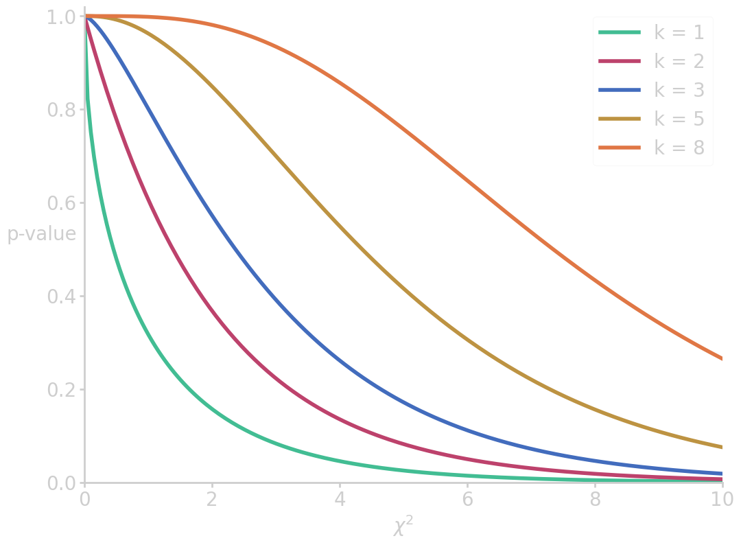
The conclusion in this example is that with a p-value of 12.75% there is not sufficient evidence to reject the null hypothesis.
Note that testing the proportion of one category can be done with the z-test. The chi-square test provides an extension of the z-test to testing several categories.
Testing homogeneity
The \(\chi^2\) test of homogeneity tests the null hypothesis that the distribution of a categorical variable is the same for several populations.
To see how the test works, let’s look at the survival data for the Titanic
| First | Second | Third | Crew | Total | |
|---|---|---|---|---|---|
| Survived | 202 | 118 | 178 | 215 | 713 |
| Died | 123 | 167 | 528 | 698 | 1516 |
| Total | 325 | 285 | 706 | 913 | 2229 |
Note that in this case we are not sampling from a population: The data are not a random sample of the people on board, rather the data represent the whole population.
Then the 325 observations about first class passengers represent 325 independent draws from a probability histogram that gives a certain chance for survival. The 285 observations about second class passengers are drawn from the probability histogram for second class passengers, which may be different. The null hypothesis says that the probability of survival is the same for all four probability histograms.
Under the \(\nullH\) assumption the survival rate is the pooled probability \(\frac{713}{713+1516} \approx 0.3199\). So the expected numbers of surviving and dying passengers are
| First | Second | Third | Crew | |
|---|---|---|---|---|
| Total | 325 | 285 | 706 | 913 |
| Survived | 202 | 118 | 178 | 215 |
| \(\nullH\)(Survived) | 103.96 | 91.16 | 225.83 | 292.05 |
| Died | 123 | 167 | 528 | 698 |
| \(\nullH\)(Died) | 221.04 | 193.84 | 480.17 | 620.95 |
The \(\chi^2\) can be calculated over all 8 cells in the table, where the degrees of freedom are given by the number of columns \(-1\) \(\times\) the number of rows \(-1\).
import numpy as np
import pandas as pd
from matplotlib import pyplot as plt

# read table above
df = pd.DataFrame(titanic_table).iloc[:, 2:].drop(1).reset_index(drop=True)
# set table names and clean up dataframe
df.columns = list(df.iloc[0])
df = df.drop(0).reset_index(drop=True)

# calculate chi2
chi2_survived = pd.DataFrame((df.iloc[1] - df.iloc[2])**2 / df.iloc[2]).T
chi2_survived_sum = chi2_survived.iloc[0].sum()
chi2_survived_red = chi2_survived_sum / (len(chi2_survived.columns)-1)

chi2_died = pd.DataFrame((df.iloc[3] - df.iloc[4])**2 / df.iloc[4]).T
chi2_died_sum = chi2_died.iloc[0].sum()
chi2_died_red = chi2_died_sum / (len(chi2_died.columns)-1)

chi2 = chi2_survived + chi2_died
chi2_sum = chi2_survived_sum + chi2_died_sum
chi2_red = chi2_survived_red + chi2_died_red

# plot chi2 statistic
plt.bar(df.columns, chi2_survived.iloc[0], label=r'$\chi^2_{\mathrm{survived}}$')
plt.bar(df.columns, chi2_died.iloc[0], label=r'$\chi^2_{\mathrm{died}}$', zorder=99)
plt.bar(df.columns, chi2.iloc[0], label=r'$\chi^2$', zorder=-1)
plt.axhline(chi2_survived_red, ls='--', c='#42bd93', zorder=100,
            label=r'$\chi^2_{\nu,\mathrm{survived}}$')
plt.axhline(chi2_died_red, ls='--', c='#bd426c', zorder=100,
            label=r'$\chi^2_{\nu,\mathrm{died}}$')
plt.axhline(chi2_red, ls='--', c='#426cbd', zorder=100,
            label=r'$\chi^2_{\nu}$')
# print(plt.rcParams['axes.prop_cycle'].by_key()['color'])
plt.legend()
filename = 'images/titanic_chi2dist.png'
plt.savefig(filename)
plt.close()

print("chi2           = {:6.4f}".format(chi2_sum))
print("chi2 (reduced) = {:6.4f}".format(chi2_red))
chi2           = 192.3435
chi2 (reduced) = 64.1145
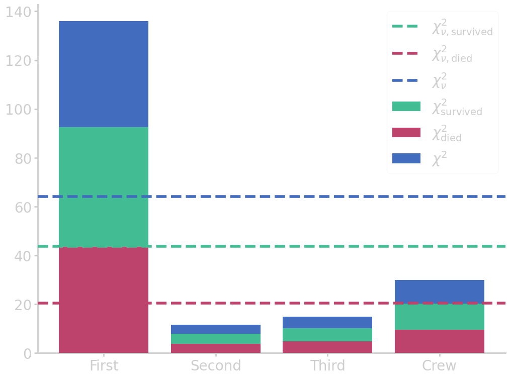
Since we obtained a very high (reduced) \(\chi^2\) statistic, the model or null hypothesis is not appropriate to describe the data. In other words, with such a high \(\chi^2\) statistic the p-value is nearly zero, which means that there is strong evidence against the null hypothesis, and \(\nullH\) should be rejected. So, the chances of survival on board the Titanic did indeed depend on the ticket class.
Testing independence
Testing independence is analogous to testing homogeneity, with only slight differences:
| Sample | Research question | \(\nullH\) | |
|---|---|---|---|
| \(\chi^2\) test of homogeneity | single categorical variable, measured on several samples | Do the groups have the same distribution of the categorical variable? | Yes |
| \(\chi^2\) test of independence | two categorical variables, measured on a single sample | Are the two categorical variables independent? | Yes |
The Analysis of Variance (ANOVA) / F-Test
Assume, we want to assess the impact of studying, homework, and peer assessment work. Our experiment randomized students into three groups and used a final exam to assess their progress.
Had we had only two groups, we could have used a two-sample t-test to study the impact. However, the generalization of this approach called ANOVA (Analysis of Variance).
Consider two hypothetical outcomes:
- the differences between multiple sample means are large relative to
the variability within the groups
- suggesting that there is a difference in treatment means
- the differences between multiple sample means are small relative to
the variability within the groups
- perhaps due to chance variability
The key idea of ANOVA is to compare the sample variance of the means to the sample variance within the group. Recall that according to the square root law (\ref{eq:sqrt_law}), the chance variability in the sample mean is smaller than the chance variability in the data. So the evidence against the null hypothesis is not immediately obvious.
We have \(k\) groups and the \(j\) th group has \(n_j\) observations
| group 1 | group 2 | \(\cdots\) | group \(k\) | average | |
|---|---|---|---|---|---|
| observation 1 | y11 | y12 | \(\cdots\) | y1\(k\) | |
| observation 2 | y21 | y22 | \(\cdots\) | y2\(k\) | |
| \(\vdots\) | \(\vdots\) | \(\vdots\) | \(\vdots\) | \(\vdots\) | |
| observation nk | yn11 | yn22 | \(\cdots\) | yn\(k\)\(k\) | |
| average | \(\bar{y}_1\) | \(\bar{y}_2\) | \(\cdots\) | \(\bar{y}_k\) | \(\bar{y}\) |
| variance | \(s^2_1\) | \(s^2_2\) | \(\cdots\) | \(s^2_k\) |
In total there are \(N = n_1 + \ldots + n_{k}\) observations. The sample mean and variance of the \(j\) th group are
\[\begin{align} \bar{y}_j&=\frac{1}{n_j}\sum_{i=1}^{n_j}{y_{ij}}\\ s^2_j& = \frac{1}{n_j-1}\sum_{i=1}^{n_j}{(y_{ij} - \bar{y}_j)^2} \end{align}\]The null hypothesis states that all group means are equal:
\begin{equation} \nullH:\quad \bar{y}_1 = \bar{y}_2 = \cdots = \bar{y}_k \end{equation}
The overall sample mean is
\begin{align} \bar{\bar{y}}&=\frac{1}{N}\sum_{j=1}^{k}{\sum_{i=1}^{n_j}{y_{ij}}} = \frac{1}{N}\sum_{j=1}^{k}{n_j\bar{y}_j} \end{align}
The total sum of squares TSS can be partitioned into components related to the effects used in the model, i.e. the sum of square treatments SST (or explained sum of squares ESS) and the sum of square errors SSE (or residual sum of squares RSS)
\[\begin{align} &\mathrm{TSS} = \mathrm{SST} + \mathrm{RSS}\\ \mathrm{TSS} &= \sum_{j}^{k}{\sum_{i}^{n_j}{(y_{ij}-\bar{\bar{y}})^2}}\\ \mathrm{SST} &= \mathrm{ESS} = \sum_{j}^{k}{\sum_{i}^{n_j}{(\bar{y}_j-\bar{\bar{y}})^2}} = \sum_{j}^{k}{n_j(\bar{y}_j-\bar{\bar{y}})^2}\\ \mathrm{SSE} &= \mathrm{RSS} = \sum_{j}^{k}{\sum_{i}^{n_j}{(y_{ij}-\bar{y}_j)^2}} = \sum_{j}^{k}{(n_j-1)s^2_j} \end{align}\]The mean squares can be calculated from sums of squares by dividing by the degrees of freedom
\[\begin{align} \mathrm{MST} &= \mathrm{EMS} = \frac{\mathrm{SST}}{k-1} = \frac{\mathrm{ESS}}{k-1}\\ \mathrm{MSE} &= \mathrm{RMS} = \frac{\mathrm{SSE}}{N-k} = \frac{\mathrm{RSS}}{N-k} \end{align}\]Since we want to compare the variation between the groups to the variation within the groups, we look at the ratio
\begin{equation}\label{eq:f_ratio} F = \frac{\mathrm{MST}}{\mathrm{MSE}} \end{equation}
Under the null hypothesis of equal group means (and group sizes) this ratio should be about 1. It will not be exactly 1 due to sampling variability:
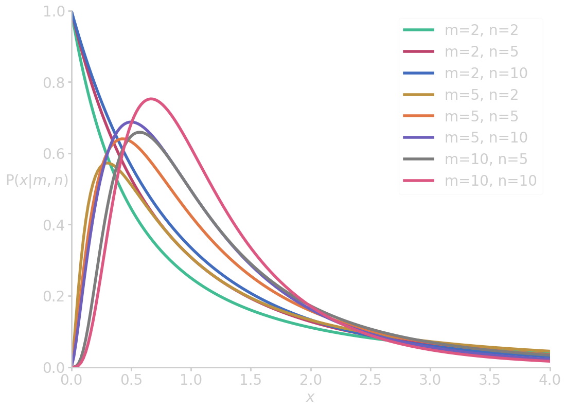
It follows a F-distribution with \(k−1\) and \(N−k\) degrees of freedom. Large values of \(F\) suggest that the variation between the groups is unusually large. We reject \(\nullH\) if \(F\) is in the right 5% tail, i.e. when the p-value is smaller than 5%.
from math import gamma
import numpy as np
import matplotlib.pyplot as plt

def F_dist(x, m, n):
    m2, n2 = m/2, n/2
    factor = m**m2 * n**n2 * gamma(m2+n2)/gamma(m2)/gamma(n2)
    pdf = factor * x**(m2-1) / (m*x + n)**(m2+n2)
    return pdf

x = np.linspace(0, 4, 200)
for m, n in zip([2, 2, 2, 5, 5, 5, 10, 10], [2, 5, 10, 2, 5, 10, 5, 10]):
    fx = F_dist(x, m, n)
    plt.plot(x, fx, label=f'm={m}, n={n}')
plt.xlim(0, 4)
plt.ylim(0, 1)
plt.ylabel('$\mathrm{P}(x| m, n)$  ', rotation=0)
plt.xlabel('$x$')
plt.legend()

filename = 'images/f_dist.png'
plt.savefig(filename)
plt.close()
return filename
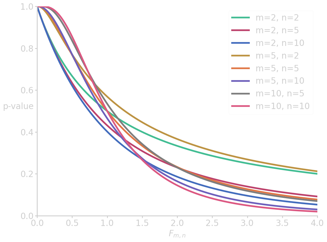
So, in the example of the impact of study methods, say, we have an F statistic of 2.49 with 3 and 38 degrees of freedom. The, the p-value is
import scipy.stats as scs
import numpy as np
import matplotlib.pyplot as plt


x = np.linspace(0, 4, 200)
for m, n in zip([2, 2, 2, 5, 5, 5, 10, 10], [2, 5, 10, 2, 5, 10, 5, 10]):
    fx = 1 - scs.f.cdf(x, m, n, loc=0, scale=1)
    plt.plot(x, fx, label=f'm={m}, n={n}')
plt.xlim(0, 4)
plt.ylim(0, 1)
plt.ylabel('p-value', rotation=0)
plt.xlabel('$F_{m,n}$')
plt.legend()

filename = 'images/p_vs_f.png'
plt.savefig(filename)
plt.close()

p = 100*(1 - scs.f.cdf(2.49, 2, 38, loc=0, scale=1))
print("p-value (ANOVA for study methods) = {:6.4f} %".format(p))
p-value (ANOVA for study methods) = 9.6344 %
which is not enough evidence to reject \(\nullH\).
The ANOVA method consists of many different components: sums of squares (SS), which have different degrees of freedom (df), and mean squares (MS). Often, it is useful to display all relevant information in a summary table
| Source | df | SS | MS | F | p-value |
|---|---|---|---|---|---|
| Treatment | k-1 | SST (or ESS) | MST (or EMS) | \(\frac{\mathrm{MST}}{\mathrm{MSE}}\) (or \(\frac{\mathrm{EMS}}{\mathrm{RMS}}\)) | |
| Error | N-k | SSE (or RSS) | MSE (or RMS) | - | |
| Total | N-1 | TSS | - | - |
The one-way ANOVA model behind the table is
\begin{equation} y_{ij} = \mu_j + \epsilon_{ij} \end{equation}
where the j-th group’s mean is \(\mu_j\) and \(\epsilon_{ij}\) are independent random error variables, e.g. measurement errors, that are normally distributed with mean 0 and common variance \(\sigma^2\). So, the null hypothesis
\begin{equation} \nullH:\quad \mu_1 = \mu_2 = \cdots = \mu_k \end{equation}
Instead of using group individual means, it is common to express the group means as deviations \(\tau_j = \mu_j - \mu\) from the grand mean \(\mu\)
\begin{equation} y_{ij} = \mu + \tau_j + \epsilon_{ij} \end{equation}
Then, the null hypothesis can be rewritten as
\begin{equation} \nullH:\quad \tau_1 = \tau_2 = \cdots = \tau_k = 0 \end{equation}
Taking \(\bar{\bar{y}}\) as estimate for \(\mu\), \(\bar{y}_j\) as estimate for \(\mu_j\), and \(\epsilon_{ij}\) as \(y_{ij}-\bar{y}_j\), and so on, we get
\begin{equation} y_{ij} = \bar{\bar{y}} + (\bar{y}_j-\bar{\bar{y}}) + (y_{ij}-\bar{y}_j) \end{equation}
It turns out that these estimates also hold for the sum of squares, which we already discussed
\[\begin{align} \sum_{j}{\sum_{i}{(y_{ij}-\bar{\bar{y}})^2}} &= \sum_{j}{\sum_{i}{(\bar{y}_j-\bar{\bar{y}})^2}} + \sum_{j}{\sum_{i}{(y_{ij}-\bar{y}_j)^2}} \\ \mathrm{TSS} &= \mathrm{SST} + \mathrm{RSS} \end{align}\]Some notes on ANOVA and the F-test
- it assumes that all the groups have the same variance \(\sigma^2\)
- this can be check visually using box-plots, or via numerical methods
- it assmues that the data are independent within and across groups
- this can be assured by randomly assigning subjects to treatments
- If the F-test rejects the null hypothesis, we can conclude that the
group means are not all equal
- we can examine all pairs of means with a two-sample t-test using \(s_{\mathrm{pooled}}=\sqrt{MSE}\)
- this involves several tests, an adjustment such as the Bonferroni adjustment is necessary (see next section)
Reproducibility and Replicability
A statistical test summarizes the evidence for an effect by reporting a single number, usually the p-value: the smaller the value, the stronger the evidence for the investigated effect. However, if a study reports a 1% p-value and call the test “highly significant”, then there is still a 1% chance to get such a highly significant even if there is no effect. For example, if we investigate if living near a power line induces cancer on a test sample of 800 subjects, then there are still 8 subjects who will show signs of an effect even if there is none, just by chance.
This is called the multiple testing fallacy or look-elsewhere effect. In the age of big data, there are so many relationships to explore that if we look them, we are bound to find some just by chance. This process is called data snooping or data dredging.
Data snooping and other problems have lead to a crisis with regard to replicability (getting similar conclusions with different samples, procedures and data analysis methods) and reproducibility (getting the same results when using the same data and methods of analysis).
Bonferroni correction
- if there are \(m\) tests, multiply the p-valuies by \(m\)
It ensures that \(\prob{\mbox{any of the m tests rejects in error}} \leq 5\%\).
The Bonferroni correction is often very restrictive, because it tries to completely eliminate the chances of a Type I error (false positive) among the \(m\) tests.
As a consequence the adjusted p-values may not be significant any more even if a noticeable effect is present.
False Discovery Rate
Alternatively to the Bonferroni correction, we can control the False Discovery Proportion (FDP)
\begin{equation} \mathrm{FDP} = \frac{\mbox{number of false discoveries}}{\mbox{total number of discoveries}} \end{equation}
where a ‘discovery’ occurs when a test rejects the null hypothesis.
Let’s assume, we test 1000 hypotheses, of which 900 are true null hypotheses and in 100 cases an alternative hypothesis is true.
Once, all hypotheses were analysed, we made 80 true discoveries and 41 false discoveries. Then, false discovery proportion is \(\frac{41}{80+41} = 0.34\).
The procedure to control the FDP at a level, say \(\alpha=5\%\), is called the Benjamini-Hochberg procedure:
- Sort the p-values \(p_1 \leq p_2 \leq \ldots \leq p_m\)
- find the largest \(k\) such that \(p_k \leq \frac{k}{m}\alpha\)
- declare discoveries fir all tests \(i\) from 1 to \(k\), and ignore all above
Splitting data
Usually in machine learning, the dataset is split into a model building dataset and a validation dataset. You may use data snooping on the model-building set to find some interesting effect.
Then, this hypothesis is tested on the validation set.
This approach requires strict discipline, because the validation set has be blinded during the exploration of the model-building dataset.
Summary of tests
| Test | Statistic | Applicability | Metric | \(\nullH\) rejection |
|---|---|---|---|---|
| z-test | \(z=\frac{\bar{X}-\mu}{\sigma/\sqrt{n}} \\\sim \mathrm{N}\) | approx. norm. dist., estimate for \(\sigma\) known | \(\mathrm{p} = \frac{1}{2}\mathrm{erfc}\left[\frac{x}{\sqrt{2}}\right] \\\in[0, 1]\) | \(p<5\%\) |
| two-sample z-test | \(z=\frac{\bar{X}_1-\bar{X}_2-\delta_{0}}{\sqrt{\sigma_1^2/n_1 + \sigma_2^2/n_2}} \\\sim \mathrm{N}\) | both samples independent, approx. norm. dist. | ||
| t-test | \(t_{n-1}=\frac{\bar{X}-\mu}{s/\sqrt{n}} \\\sim \mathrm{T}\) | possibly norm. dist., but \(\sigma\) unknown | \(\mathrm{p} = 1-\int^{x}{T(u)\mathrm{d}u} \\\in[0, 1]\) | \(p<5\%\) |
| two-sample t-test | \(t=\frac{\bar{X}_1-\bar{X}_2-\delta_{0}}{\sqrt{s_1^2/n_1 + s_2^2/n_2}} \\\sim \mathrm{T}\) | both samples independent, approx. norm. dist. | ||
| ANOVA / F-test | \(\mathrm{F}_{1}= \frac{\mbox{MST}}{\mbox{MSE}}\\ = \frac{\frac{1}{k-1}\sum_{j}^{k}{n_j(\bar{y}_j-\bar{\bar{y}})^2}}{\frac{1}{N-k}\sum_{j}^{k}{(n_j-1)s^2_j}} \\\sim \mathrm{F}\) | all groups have same variance \(\sigma^2\), data are independent within and across groups | \(\mathrm{p} = 1-\int^{x}{F(u)\mathrm{d}u} \\\in[0, 1]\) | \(p<5\%\) |
| \(\chi^2\) test | \(\chi^2=\sum\frac{(d^{(i)}_\mathrm{obs}-d^{(i)}_\nullH)^2}{d^{(i)}_\nullH}=\sum\frac{(d^{(i)}_\mathrm{obs}-d^{(i)}_\nullH)^2}{\sigma_{i}^2}\) | categorical data, contingency table, \(\nu =\) #observations \(-\) #parameters | \(\chi_{\nu}^{2} = \frac{\chi^2}{\nu}\) | \(1 << \chi^2_{\nu} << 1\) |
Resources
For the examples in this post, I tried to keep the imports of modules
to a minimum, however for the sake of keeping the snippets short and
avoiding code repetition, I used utils.py to store a function for
calculating binomial coefficients and formatting print statements, as
well as the random number generation algorithm MT19937: