Some notes on quantum computing
Recently, I received note that IBM has several quantum processors which are available to the public for free. As computing and programming is a passion of mine and I like to try new things, I decided to give them a try. As anticipated, programming on such a chip is no easy task, because the underlying physics is completely different to conventional processors. So, here is my attempt of connecting the physics of the quantum realm with computing…
Table of Contents
\( \newcommand\cvec[1]{\begin{pmatrix}#1\end{pmatrix}} \newcommand\bra[1]{\langle#1\rvert} \newcommand\ket[1]{\lvert#1\rangle} \newcommand\braket[2]{\langle#1\rvert\,#2\rangle} \newcommand\ketbra[2]{\lvert#1\rangle\langle#2\rvert} \newcommand{\frasq}{\frac{1}{\sqrt{2}}} \)
Basics: Quantum Computing and Circuits
Quantum computation can be seen as an extension of classical computing (as designed by Alan Turing around 1936) into the “Multiverse”. Quantum computers are/will be capable of new modes of information processing of which classical computers are fundamentally incapable.
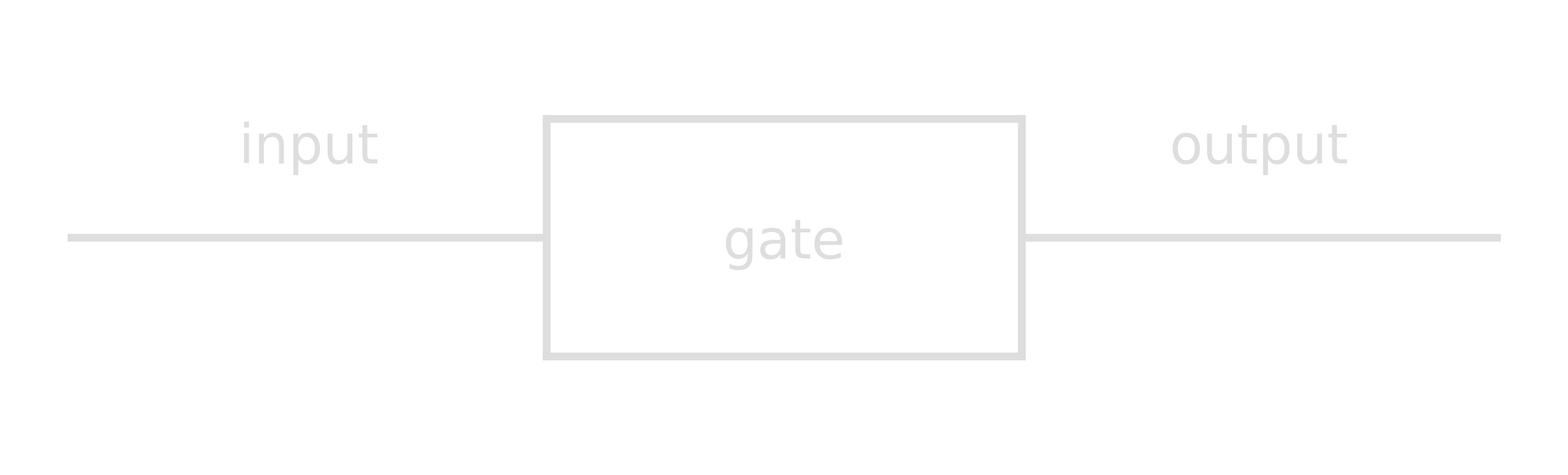
The concept of computation is an explicit form of a physical system which processes information.
| Computation | Physics | Example |
|---|---|---|
| computer | physical system | measuring instrument |
| computation | motion | experiment, measurement |
| input | initial state | preparation |
| rules | laws of motion | |
| output | final state | outcome |
The basis of a physical quantum system is called a qubit. A qubit describes a minimal physical (quantum) system with two base states of a quantum observable (mathematically described by a matrix whose eigenvalues are measureable outcomes of the observable).
Note that quantum observables often have a discrete set of measureable outcomes, i.e. the spectrum of some observable might be
\begin{equation} Sp( \hat{\phi} ) = {x=n\frac{\pi}{2}\ |\ 0 \leq x \leq 2\pi\ \forall\ n \in \mathbb{Z} } \end{equation}
rather than a continuous set such as
\begin{equation} Sp( \hat{\theta} ) = {x \in \mathbb{R}\ |\ 0 \leq x \leq 2\pi } \end{equation}
Qubits and Quantum States
Classical states for computation are either 1 or 0. In quantum mechanics however, states can also be in superposition, i.e. simultaneously 1 and 0, which allows to perform calculations on many states at the same time and promises a speed-up in comparison to classical algorithms. In fact, some quantum algorithms indeed speed up computations exponentially.
Unfortunately, there is a catch. Once a quantum state is measured, it collapses into either states. This complicates the designing of quantum algorithms. Interference effects can be used to mitigate these problems.
The designing of quantum algorithms therefore requires some basic knowledge of quantum mechanics. The mathematical description of quantum states is very condensed, but actually very easy to understand.
Dirac notation
The Dirac notation is typically used to describe quantum states. Also known as Bra-Ket notation, it is defined as follows. Let \(a\), \(b\) \(\in \mathbb{C}\),
Ket:
\begin{equation}\label{eq:ket-notation} \ket{a} = \cvec{a_1 \ a_2} \end{equation}
Bra:
\begin{equation}\label{eq:bra-notation} \bra{b} = \ket{b}^{\dagger} = \cvec{b_1 \ b_2}^{\dagger} = \cvec{b_1^{\ast}&b_2^{\ast}} \end{equation}
where the complex conjugate is \(b^{\ast}=c-id\) for the complex number \(b=c+id\).
Bra-Ket:
\begin{equation}\label{eq:bra-ket-notation} \braket{b}{a} = \braket{a}{b}^{\ast} = a_1b_1^{\ast} + a_2b_2^{\ast} \end{equation}
Ket-Bra:
\begin{equation}\label{eq:ket-bra-notation} \ketbra{a}{b} = \cvec{a_1b_1^{\ast} & a_1b_2^{\ast} \ a_2b_1^{\ast} & a_2b_2^{\ast}} \end{equation}
Additionally, we define the states \(\ket{0}=\cvec{1 \ 0}\) and \(\ket{1}=\cvec{0 \ 1}\), which are orthogonal, i.e. \(\braket{0}{1}=0\).
All quantum states are also defined to be normalized, i.e. \(\braket{\psi}{\psi}=1\). For instance, \(\ket{\psi}=\frasq(\ket{0}+\ket{1})=\cvec{1/\sqrt{2} \ 1/\sqrt{2}}\), and \(\cvec{1/\sqrt{2}&1/\sqrt{2}}\cvec{1/\sqrt{2} \ 1/\sqrt{2}}=\frac{1}{2}+\frac{1}{2}=1\).
Measurements
We usually choose orthogonal bases to describe and measure quantum states. During a measurement onto the basis \({\ket{0}, \ket{1}}\), the state will collapse to either component which are the eigenstates of \(\sigma_z\). We call this a z-measurement.
There are arbitrarily many bases, but the most common ones corresponding to the eigenstates of
- \(\sigma_x\):
\begin{align}\label{eq:x-eigenstates}
\ket{+} &= \frasq (\ket{0} + \ket{1})
\ket{-} &= \frasq (\ket{0} - \ket{1})
\end{align}
- \(\sigma_y\):
\begin{align}\label{eq:y-eigenstates}
\ket{+i} &= \frasq (\ket{0} + i\ket{1})
\ket{-i} &= \frasq (\ket{0} - i\ket{1})
\end{align}
The probability that a state \(\ket{\psi}\) collapses during a projective measurement onto the basis \({\ket{x}, \ket{x^{\dagger}}}\) to the state \(\ket{x}\) is given by the Born rule:
\[\begin{align}\label{eq:born-rule} P(x) &= |\braket{x}{\psi}|^{2} \\ \sum_{i} P(x_i) &= 1 \end{align}\]For example: \(\ket{\psi}=\frac{1}{\sqrt{3}}(\ket{0}+\sqrt{2}\ket{1})\) is measured in the basis \({\ket{0}, \ket{1}}\):
\[\begin{align} &P(0) = |\braket{0}{\frac{1}{\sqrt{3}}(\ket{0}+\sqrt{2}\ket{1})}|^{2} = |\frac{1}{\sqrt{3}}\braket{0}{0} + \sqrt{\frac{2}{3}}\braket{0}{1}|^{2} = |\frac{1}{\sqrt{3}} + \sqrt{\frac{2}{3}} \cdot 0|^{2} = \frac{1}{3} \\ \rightarrow\quad&P(1) = 1 - P(0) = \frac{2}{3} \end{align}\]Another example: \(\ket{\psi}=\frasq(\ket{0}-\ket{1})\) is measured in the basis \({\ket{+}, \ket{-}}\):
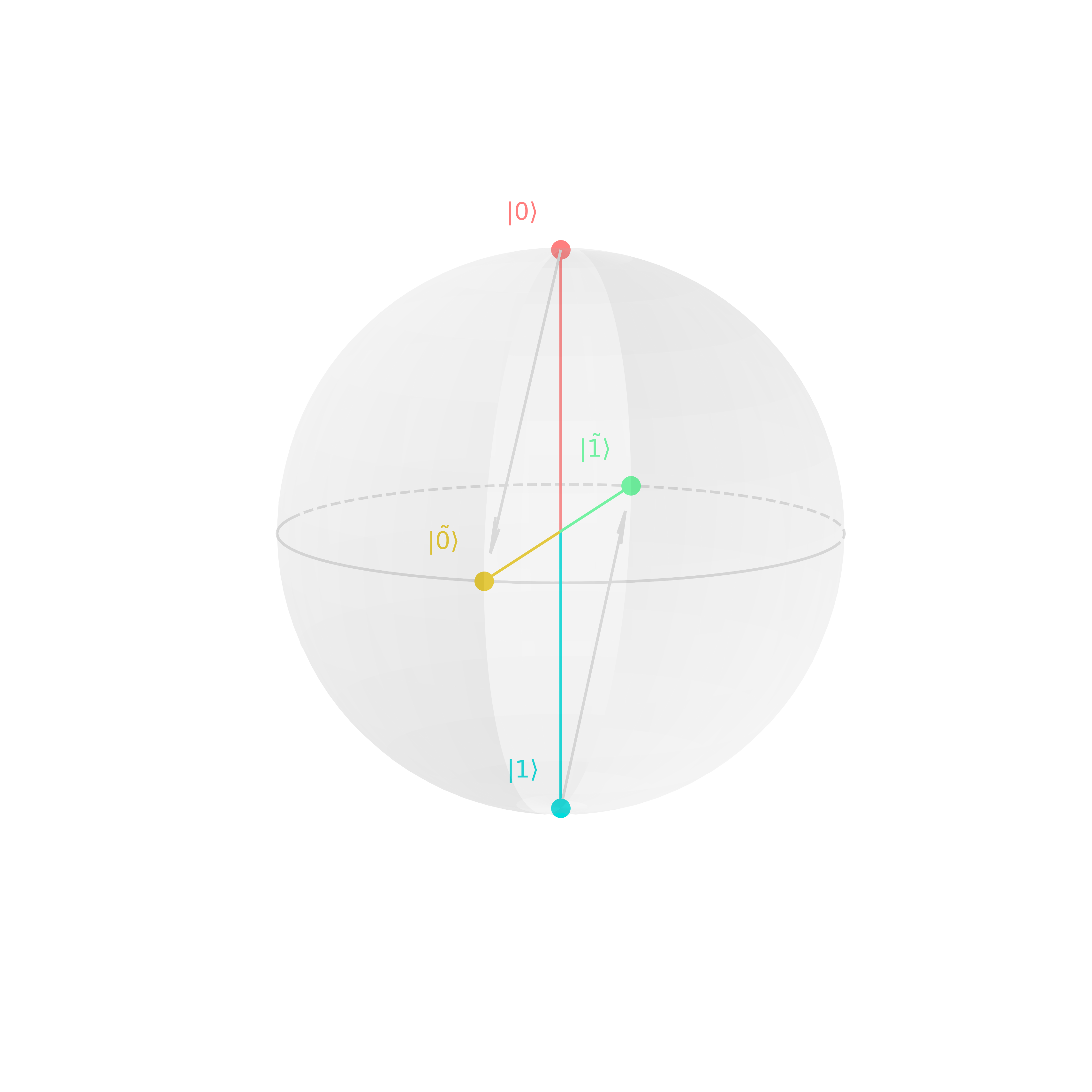
\[\begin{align} P(+) &= |\braket{+}{\psi}|^{2} = |\frasq(\bra{0}+\bra{1}) \cdot \frasq(\ket{0}-\ket{1})|^{2} \\ &= \frac{1}{4}|\braket{0}{0}-\braket{0}{1}+\braket{1}{0}-\braket{1}{1}|^{2} = \frac{1}{4}|1 - 0 + 0 - 1|^{2} = 0 \\ \rightarrow\quad P(-) &= 1 - P(+) = 1 \end{align}\]The latter example makes immediate sense if we inspect the so-called Bloch sphere, which illustrates (pure) states of a two-level quantum mechanical system, i.e. qubit, as points on a sphere in the projective Hilbert space (mathematically also known as the Riemann sphere). We can write an arbitrary, normalized, pure state as
\begin{equation} \ket{\psi} = \cos{\frac{\theta}{2}}\ket{0} + e^{i\phi}\sin{\frac{\theta}{2}}\ket{1} \end{equation}
where \(\phi\in[0, 2\pi]\) describes the relative phase and \(\theta\in[0, \pi]\) determines the probability to measure the eigenstates of \(\sigma_z\):
\[\begin{align} P(\ket{0}) &= \cos^2{\frac{\theta}{2}}\\ P(\ket{1}) &= \sin^2{\frac{\theta}{2}} \end{align}\]All normalized pure states can be illustrated as Bloch vectors on the surface of the Bloch sphere with radius \(|\mathbf{r}|=1\):
\begin{equation}\label{eq:bloch-vector} \mathbf{r} = \cvec{\sin{\theta}\cos{\phi}\\sin{\theta}\sin{\phi}\\cos{\theta}} \end{equation}
The coordinates of the Bloch vectors of the eigenstates of \(\sigma_z\), \(\sigma_x\), and \(\sigma_y\) respectively are:
\[\begin{align} \ket{0}: \quad&\theta=0,\ \phi\ \text{arbitrary}\quad\rightarrow\quad\mathbf{r} = \cvec{0\\0\\1}\\ \ket{1}: \quad&\theta=\pi,\ \phi\ \text{arbitrary}\quad\rightarrow\quad\mathbf{r} = \cvec{0\\0\\-1}\\ \ket{+}: \quad&\theta=\frac{\pi}{2},\ \phi = 0\quad\rightarrow\quad\mathbf{r} = \cvec{1\\0\\0}\\ \ket{-}: \quad&\theta=\frac{\pi}{2},\ \phi = \pi\quad\rightarrow\quad\mathbf{r} = \cvec{-1\\0\\0}\\ \ket{+i}:\quad&\theta=\frac{\pi}{2},\ \phi = \frac{\pi}{2}\quad\rightarrow\quad\mathbf{r} = \cvec{0\\1\\0}\\ \ket{-i}:\quad&\theta=\frac{\pi}{2},\ \phi = \frac{3\pi}{2}\quad\rightarrow\quad\mathbf{r} = \cvec{0\\-1\\0} \end{align}\]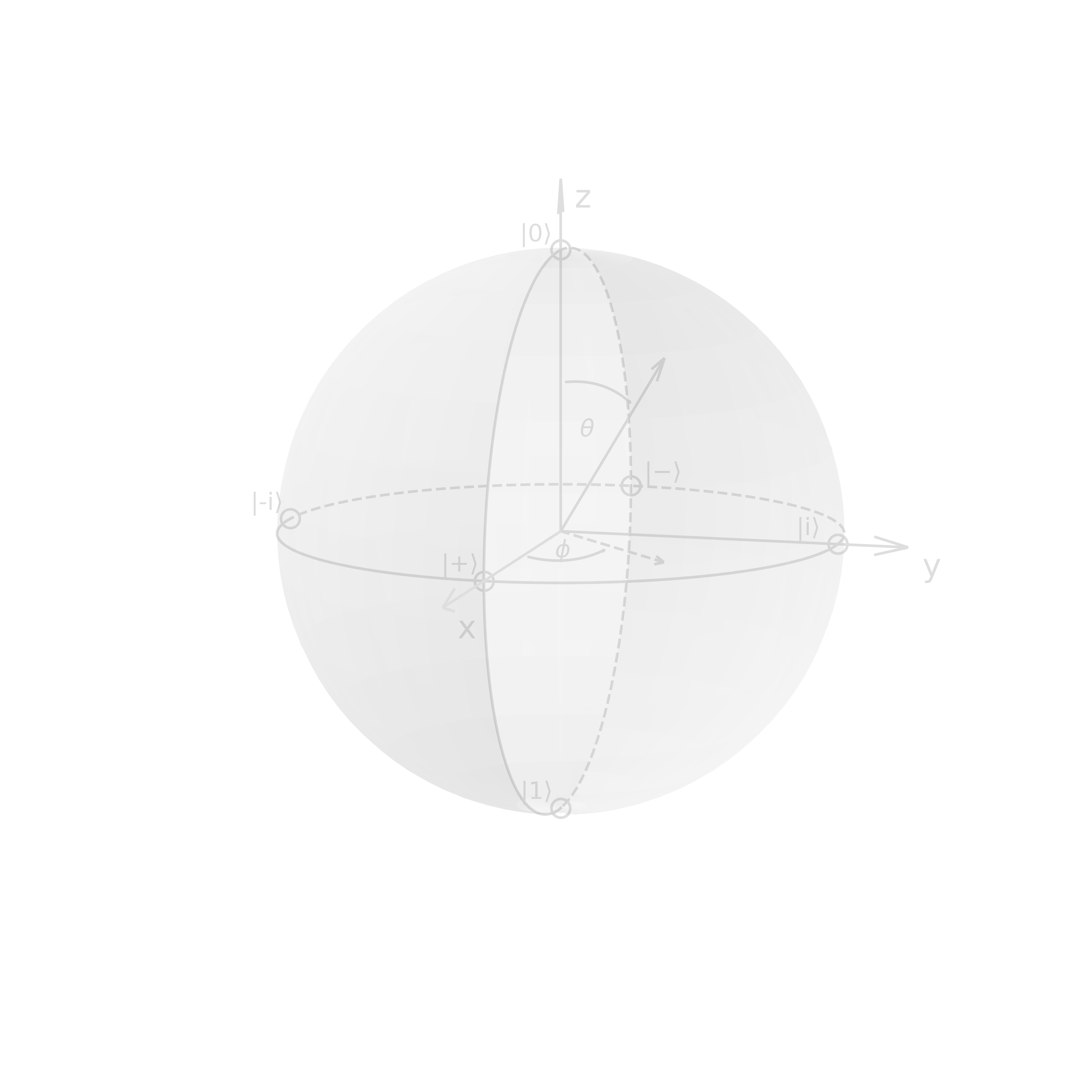
Note that on the bloch sphere angles are twice as big as in the Hilbert space, e.g. \(\ket{0}\) & \(\ket{1}\) are orthogonal, but on the Bloch sphere their angle is \(\pi\) or \(180^\circ\). Z-measurements correspond to a projection onto the z-axis, and analogously for the x and y-axes.
Quantum circuits
Circuit models are a sequence of operators which carry out elementary computations. These operators are called gates.
Single qubit gates
A classical example of a single state gate is the NOT gate which turns states into their complementary state. For quantum states, gates are represented by unitary matrices, as quantum theory is unitary. Any quantum operator can be uniquely written as a linear combination of the identity matrix and the so-called Pauli matrices:
\[\begin{align} \sigma_z &= \cvec{1&0\\0&-1} = \ketbra{0}{0} - \ketbra{1}{1}\\ \sigma_y &= \cvec{0&-i\\i&0} = \ketbra{i}{i} - \ketbra{-i}{-i} = i\ketbra{1}{0} - i\ketbra{0}{1}\\ \sigma_x &= \cvec{0&1\\1&0}\ = \ketbra{+}{+} - \ketbra{-}{-} = \ketbra{0}{1} + \ketbra{1}{0} \end{align}\]The \(\sigma_x\) gate is a bit-flip, or NOT gate, as it acts as a rotation around the x-axis by \(\pi\).
\[\begin{align} \sigma_x \ket{0} &= \cvec{0&1\\1&0}\ \cvec{1\\0} = \cvec{0\\1} = \ket{1}\\ \sigma_x \ket{1} &= (\ketbra{0}{1} + \ketbra{1}{0})\cdot\ket{0} = \ket{0}\braket{1}{1} + \ket{1}\braket{0}{1} = \ket{0} \end{align}\]The \(\sigma_z\) gate acts as a rotation around the z-axis by \(\pi\) and is therefore a phase-flip operator.
\[\begin{align} \sigma_z \ket{+} &= \cvec{1&0\\0&-1}\ \frasq\cvec{1\\1} = \frasq\cvec{1\\-1} = \ket{-}\\ \sigma_z \ket{-} &= (\ketbra{0}{0} - \ketbra{1}{1})\cdot\ket{-} = \frasq(\ket{0}+\ket{1}) = \ket{+} \end{align}\]The \(\sigma_y\) gate acts as a rotation around the y-axis by \(\pi\) and encompasses a bit and phase flip.
\begin{equation} \sigma_y = i\,\sigma_x\sigma_z \end{equation}
However, the perhaps most important gate for quantum computing is the Hadamard gate
\begin{equation}\label{eq:Hadamard-operator} H = \frasq\cvec{1&1 \ 1&-1} = \frasq (\ketbra{0}{0} + \ketbra{0}{1} + \ketbra{1}{0} - \ketbra{1}{1}) = \frasq (\sigma_z + \sigma_x) \end{equation}
It is used to change between the x and z basis and therefore creates a superposition
\[\begin{align} H\ket{0} &= \frasq\cvec{1\\1} = \ket{+}\\ H\ket{1} &= \frasq (\ketbra{0}{0} + \ketbra{0}{1} + \ketbra{1}{0} - \ketbra{1}{1})\cdot\ket{1} = \frasq(\ket{0}-\ket{1}) = \ket{-}\\ H\ket{+} &= \ket{0}\\ H\ket{-} &= \ket{1} \end{align}\]Similarly the S-gate \(S=\cvec{1&0 \ 0&i}\) can be used to switch between the x and y bases, as it adds \(\pi/2\) to the phase \(\phi\): \(S\ket{+}=\ket{i}\) and \(S\ket{-}=\ket{-i}\).
Multipartite quantum states
We use tensor products to describe multiple states:
\begin{equation}\label{eq:multipartite-states} \ket{a}\otimes\ket{b} = \cvec{a_1 \ a_2}\otimes\cvec{b_1 \ b_2} = \cvec{a_1b_1 \ a_1b_2 \ a_2b_1 \ a_2b_2} \end{equation}
For example, if a system A is in state \(\ket{1}_{A}\) and a system B is in state \(\ket{0}_{B}\), then the bipartite state is \(\ket{10}_{AB}=\ket{1}_A\otimes\ket{0}_B=\cvec{0&0&1&0}^{T}\). Note that states of this form are called uncorrelated, but there are also bipartite states that cannot be written as \(\ket{\psi}_A\otimes\ket{\psi}_B\). Such states are correlated and sometimes even entangled (very strong correlation), e.g. a so-called Bell state
\begin{equation} \ket{\psi}^{(00)}_{AB} = \frasq(\ket{00}_{AB}+\ket{11}_{AB}) = \frasq\cvec{1 \ 0 \ 0 \ 1} \end{equation}
used for teleportation, cryptography, Bell tests, etc.
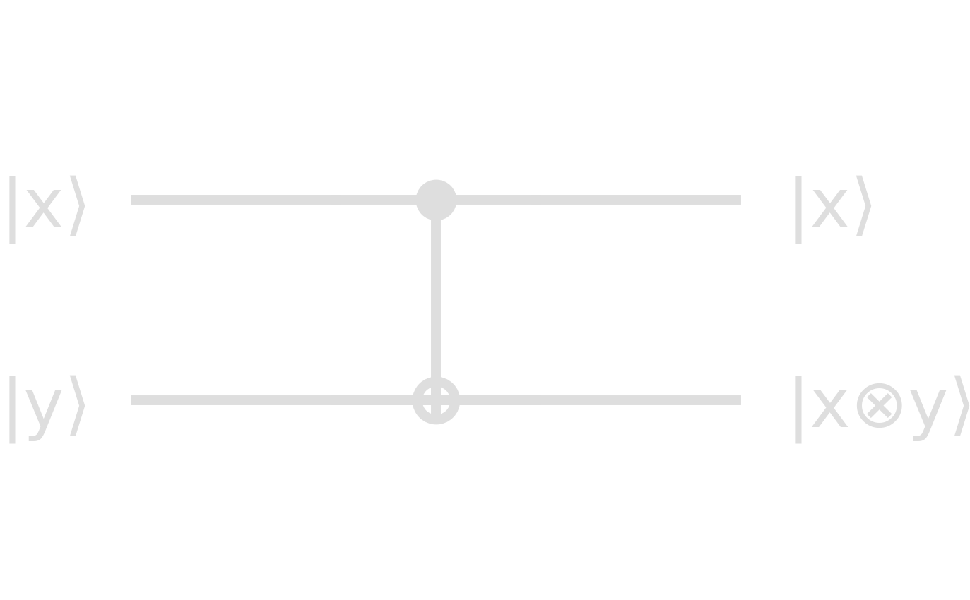
Two-qubit gates
A classical example of a two-state gate is the XOR gate which irreversibly turns states into 1 iff they differ. In quantum theory however, we only consider unitary operations and therefore reversible gates. An example of a quantum two-state gate is the CNOT gate:
\begin{equation}\label{eq:CNOT} \text{CNOT} = \cvec{1&0&0&0\0&1&0&0\0&0&0&1\0&0&1&0} = \ketbra{00}{00} + \ketbra{01}{01} + \ketbra{10}{11} + \ketbra{11}{10} \end{equation}
\[\begin{align} \text{CNOT}\cdot\ket{00}_{xy}=\text{CNOT}\cdot\cvec{1&0&0&0}^{T}=\cvec{1&0&0&0}^{T}=\ket{00}_{xy}\\ \text{CNOT}\cdot\ket{10}_{xy}=\text{CNOT}\cdot\cvec{0&0&1&0}^{T}=\cvec{0&0&0&1}^{T}=\ket{11}_{xy} \end{align}\]This gate represents a reversible version of the XOR gate. Its circuit component looks like
| input | output | ||
|---|---|---|---|
| x | y | x | x ⊗ y |
| 0 | 0 | 0 | 0 |
| 0 | 1 | 0 | 1 |
| 1 | 0 | 1 | 1 |
| 1 | 1 | 1 | 0 |
Moreover, we can show that every function \(f\) can be described by a reversible circuit, and therefore quantum circuits can perform all functions that can be calculated classically.
Entanglement
If a (pure) state \(\ket{\psi}_{AB}\) on systems A, B cannot be written as \(\sum_{i,j} c_{ij}\ket{i}_A\otimes\ket{j}_B\) with all vector components \(c_{ij} \in \mathbb{R}\) and \(c_{ij}=c_{i}^{A}c_{j}^{B}\) such that \(\ket{\psi}_A=c_{i}^{A}\ket{i}_A\) and \(\ket{\phi}_B=c_{j}^{B}\ket{j}_B\), it is entangled. For a two-qubit system it is sufficient to satisfy \(\text{det}(c_{ij})=0\) or \(c_{00}c_{11}=c_{01}c_{10}\). There are four so-called Bell states which are maximally entangled and build an orthonormal basis
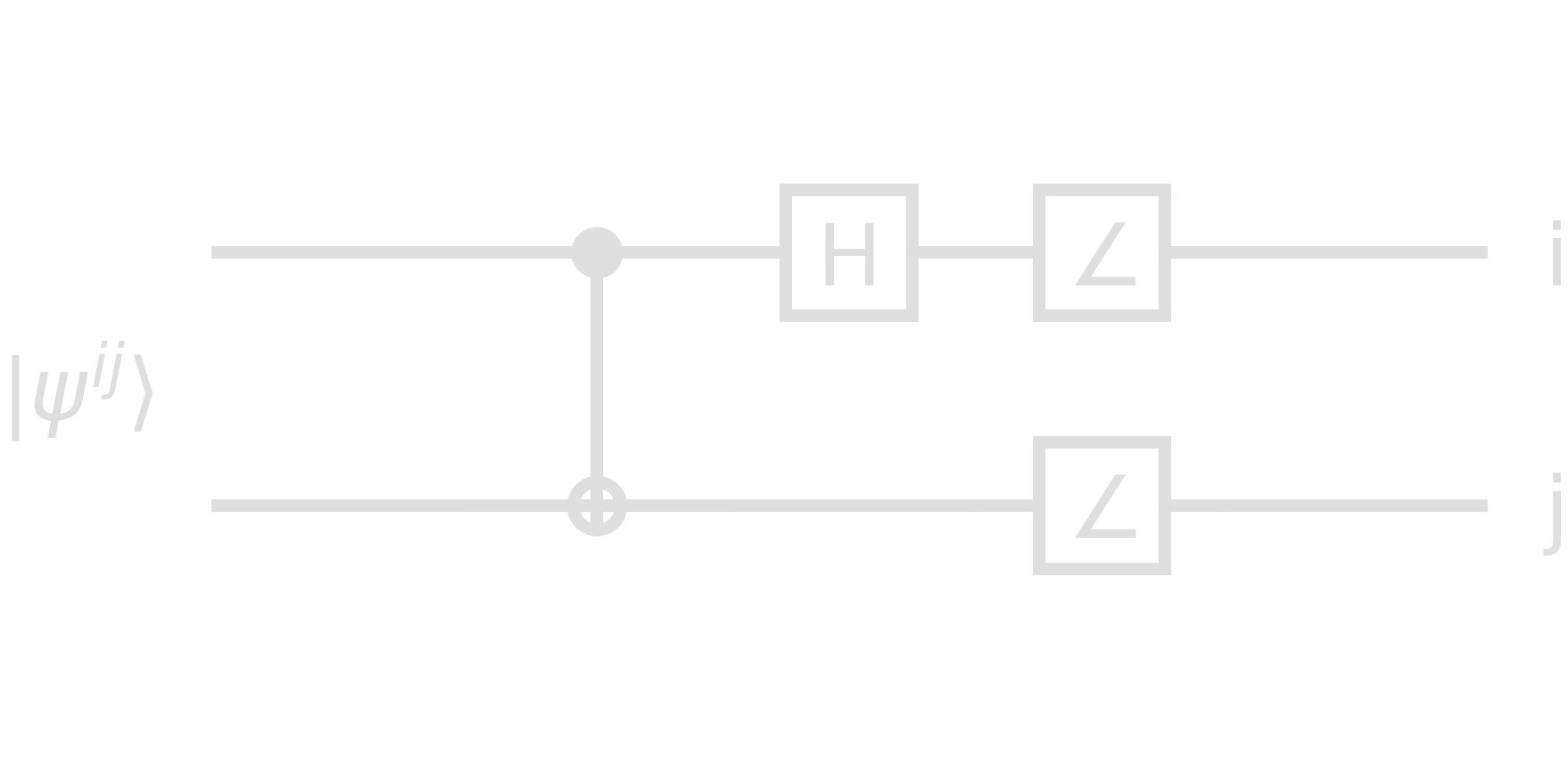
\[\begin{align}\label{eq:bell_states} \ket{\psi^{00}} &= \frasq(\ket{00}+\ket{11})\\ \ket{\psi^{10}} &= \frasq(\ket{00}-\ket{11})\\ \ket{\psi^{01}} &= (\ket{01}-\ket{10})\\ \ket{\psi^{11}} &= (\ket{01}+\ket{10}) \end{align}\]In general, we can write \(\ket{\psi^{ij}}=(\mathbb{1}\otimes\sigma^j_x\cdot\sigma^i_z)\ket{\psi^{00}}\). The creation of Bell states is therefore a relatively simple circuit, combining the Hadamard with a CNOT gate:
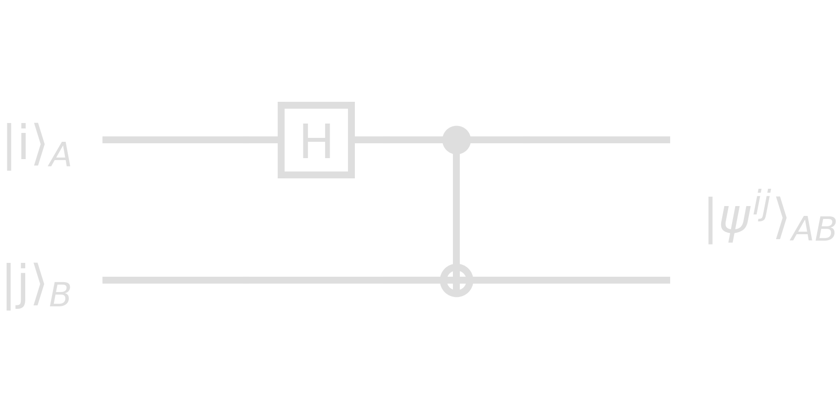
The outputs of this circuit are as expected:
| \(\ket{ij}_{AB}\) | \(H_A\otimes\mathbb{1}\ket{ij}_{AB}\) | \(\ket{\psi^{ij}}\) |
|---|---|---|
| \(\ket{00}\) | \((\ket{00}+\ket{10}) / \sqrt{2}\) | \(\ket{00}+\ket{11} / \sqrt{2} = \ket{\psi^{00}}\) |
| \(\ket{01}\) | \((\ket{01}+\ket{11}) / \sqrt{2}\) | \(\ket{01}+\ket{10} / \sqrt{2} = \ket{\psi^{01}}\) |
| \(\ket{10}\) | \((\ket{00}-\ket{10}) / \sqrt{2}\) | \(\ket{00}-\ket{11} / \sqrt{2} = \ket{\psi^{10}}\) |
| \(\ket{11}\) | \((\ket{01}-\ket{11}) / \sqrt{2}\) | \(\ket{01}-\ket{10} / \sqrt{2} = \ket{\psi^{11}}\) |
The reversed circuit therefore allows for measurements of Bell states. The last gates in the following circuit plot denotes a measurement of the quantum states which result in classical ouputs \(i\) and \(j\).
Teleportation
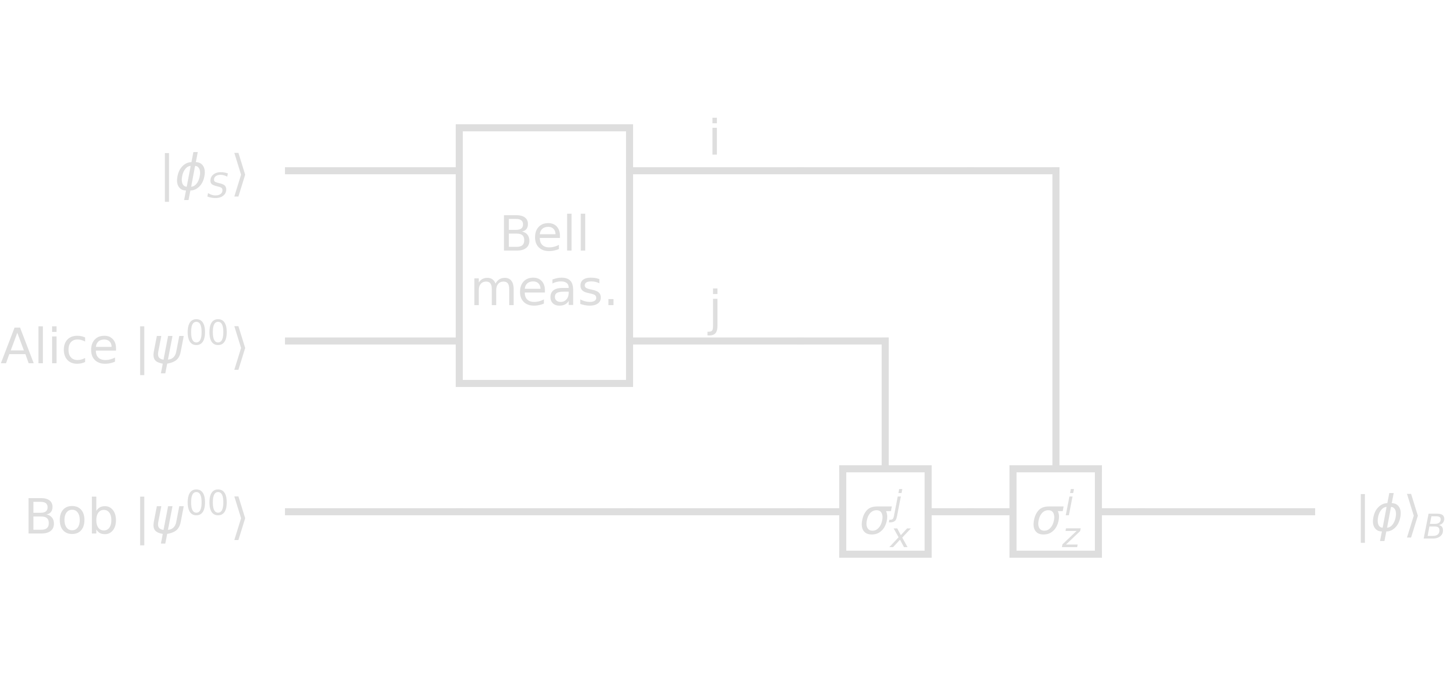
Quantum teleportation is a topic which often causes confusion in news articles due to the lack of specificity. Quantum teleportation is an instantaneous transmission of neither energy nor matter, but quantum information. It tackles a quite simple idea: Alice wants to send her (unknown/secret) state \(\ket{\phi}_S=\alpha\ket{0}_S+\beta\ket{1}_S\) to Bob. She can only send him two classical bits though. They both share the maximally entangled state \(\ket{\psi^{00}}_{AB}=\frasq(\ket{00}_{AB}+\ket{11}_{AB})\).
The initial state of the total system is therefore
\[\begin{align} \ket{\phi}_S\otimes\ket{\psi^{00}}_{AB} =& \frasq\left(\alpha\ket{000}_{SAB} + \alpha\ket{011}_{SAB} + \beta\ket{100}_{SAB} + \beta\ket{111}_{SAB}\right)\\ =&\frac{1}{2}\left[ \ket{\psi^{00}}_{SA}\otimes\ket{\phi}_B + \ket{\psi^{01}}_{SA}\otimes(\sigma_x\ket{\phi}_B)\\ + \ket{\psi^{10}}_{SA}\otimes(\sigma_z\ket{\phi}_B) + \ket{\psi^{11}}_{SA}\otimes(\sigma_x\sigma_z\ket{\phi}_B) \right] \end{align}\]The protocol works as follows:
- Alice performs a measurement on S and A in the Bell basis.
- She sends her classical outputs \(i\), \(j\) to Bob.
- Bob applies \(\sigma^i_z\sigma^j_x\) to his qubit and gets \(\ket{\phi}\).
| 1 | 2 | 3 | ||
|---|---|---|---|---|
| Alice's measurement | Bob's state | Alice sends | Bob applies gates | Bob's final state |
| \(\ket{\psi^{00}}\) | \(\ket{\phi}_B\) | 0, 0 | \(\mathbb{1}\) | \(\ket{\phi}_B\) |
| \(\ket{\psi^{01}}\) | \(\sigma_x\ket{\phi}_B\) | 0, 1 | \(\sigma_x\) | \(\ket{\phi}_B\) |
| \(\ket{\psi^{10}}\) | \(\sigma_z\ket{\phi}_B\) | 1, 0 | \(\sigma_z\) | \(\ket{\phi}_B\) |
| \(\ket{\psi^{11}}\) | \(\sigma_x\sigma_z\ket{\phi}_B\) | 1, 1 | \(\sigma_z\sigma_x\) | \(\ket{\phi}_B\) |
Note that Alice’s state collapsed during the measurement, so she does not have the initial state \(\ket{\phi}\) anymore. This is expected due to the no-cloning theorem, as she cannot copy her state, but just send her state to Bob when destroying her own.
Q-Sphere
The Bloch sphere can only illustrate the state of 1 qubit. For multiple qubits we use the Q-sphere.
Q-sphere for a single qubit:
- the north pole represents state \(\ket{0}\) and the south pole \(\ket{1}\)
- the size of the points is proportional to the probability of measuring the respective state
- colors are used to indicate relative phases compared to \(\ket{0}\)
For n qubits, there are \(2^{n}\) basis states, e.g. for \(n=3\) we have
\begin{equation} {\ket{000}, \ket{001}, \ket{010}, \ket{100}, \ket{011}, \ket{101}, \ket{110}, \ket{111}} \end{equation}
On the Q-sphere, these states are equally distributed points: \(0^{\otimes n}\) is on the north pole, \(1^{\otimes n}\) on the south pole, and all other states equally distributed on parallel circles on the sphere, their latitude increasing from north to south with increasing number of 1s.
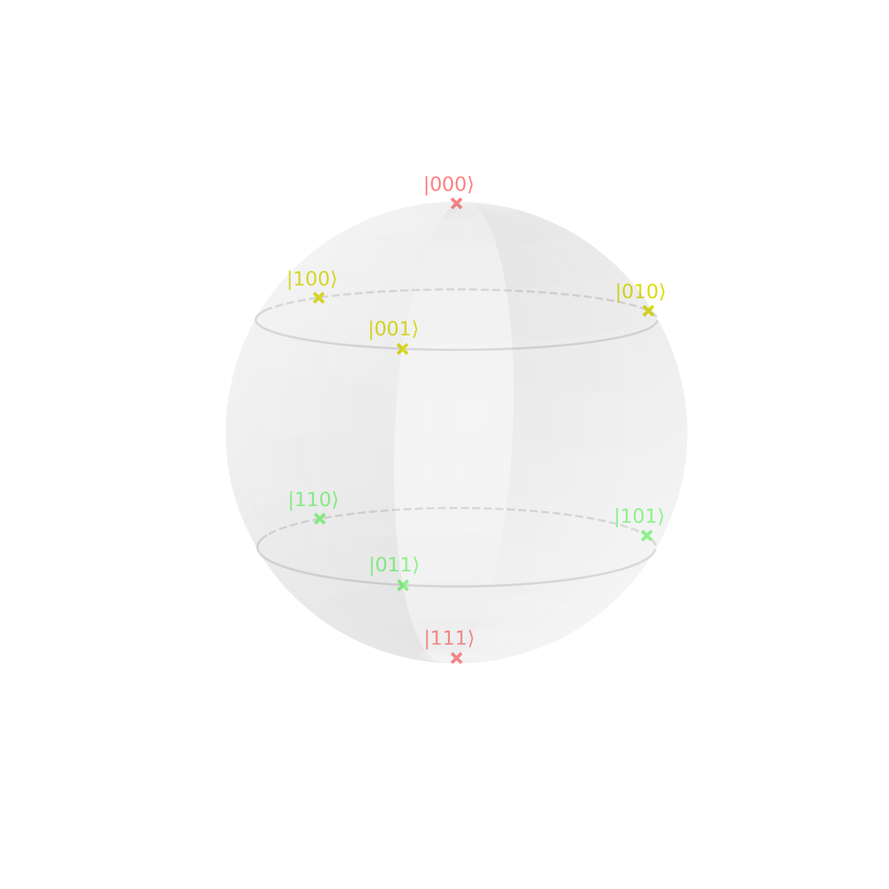
The relative phase to \(0^{\otimes n}\) determine the color. For example:
\[\begin{align} \ket{\psi} &= \frasq \cdot (\frasq\ket{000} - \frasq\ket{011} + i\cdot\ket{101})\\ &\left\{ \begin{array}{lll} \ket{000}&: \quad e^{i\phi} = 1 \quad\rightarrow\quad \color{salmon}{\phi=0^\circ}\\ -\ket{011}&: \quad e^{i\phi} = -1 \,\,\rightarrow\quad \color{turquoise}{\phi=180^\circ} \\ i\cdot\ket{101}&:\quad e^{i\phi} = i \quad\rightarrow\quad \color{yellowgreen}{\phi=90^\circ} \end{array} \right. \end{align}\]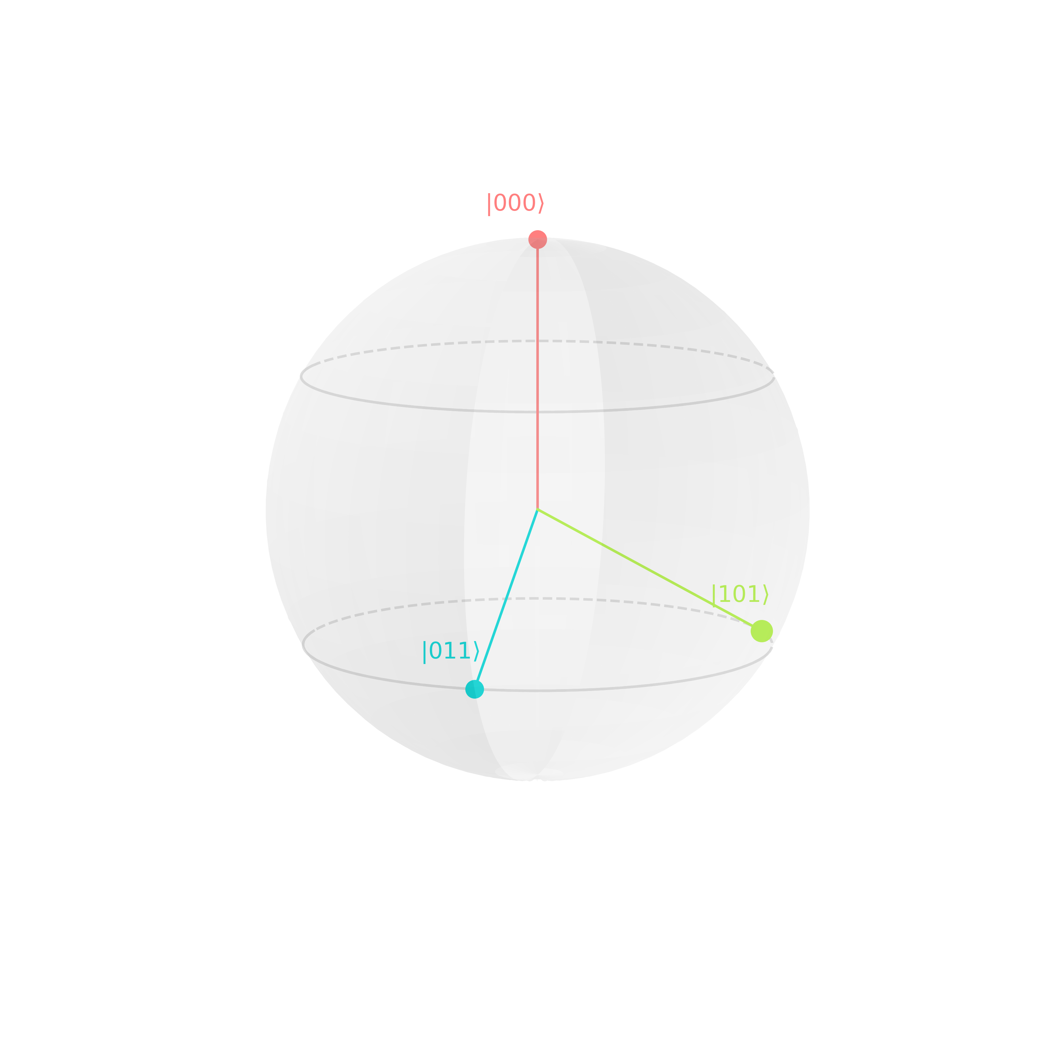
Quantum Algorithms
An algorithm is a hardware-independent specification of a computation which describes a solution to some computational task. Quantum algorithms use information processing modes which are not possible to perform with simple classical computers.
Deutsch-Jozsa algorithm
The Deutsch-Jozsa algorithm is the probably simplest of all quantum algorithms. It solves the problem of determining a function property with minimal number of queries to an oracle.
Quantum oracles
Assume we have access to an oracle, a physical device for instance which we cannot inspect, but we can pass queries to and receive answers from it. On a classical computer, such an oracle is given by a function \(f: {0, 1}^{n} \rightarrow {0, 1}^{m}\). On a quantum computer, the oracle must be reversible:
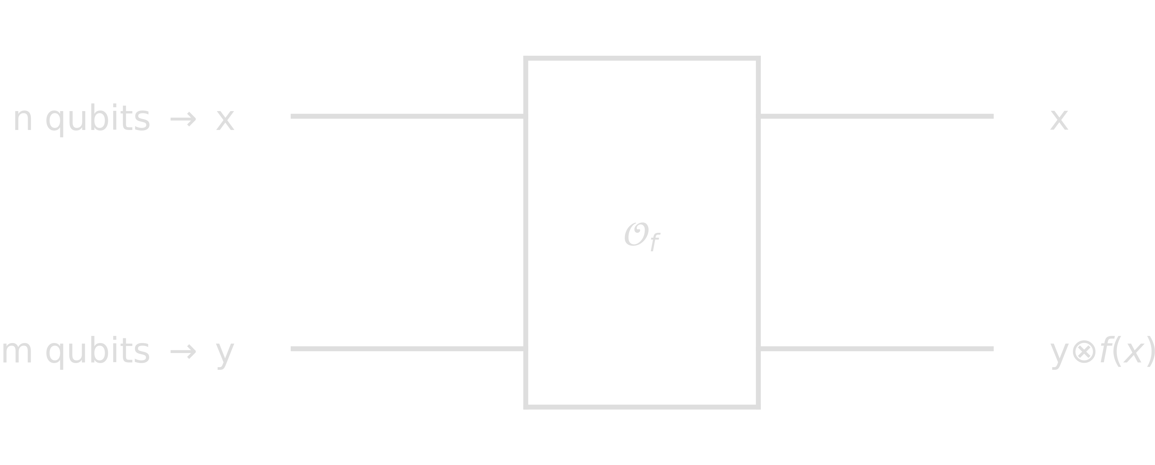
If one wants the oracle to evaluate the function \(f(x)\), the auxiliary input \(y\) simply needs be initialized as 1. The operator \(\mathcal{O}_f\) (also called bit oracle) can be seen as a unitary map of the form \(\mathcal{O}_f\ket{x}\ket{y}=\ket{x}\ket{y\otimes f(x)}\). For \(f: {0, 1}^{n} \rightarrow {0, 1}\), we can alternatively construct an oracle \(\mathcal{U}_f\) (also called phase oracle):
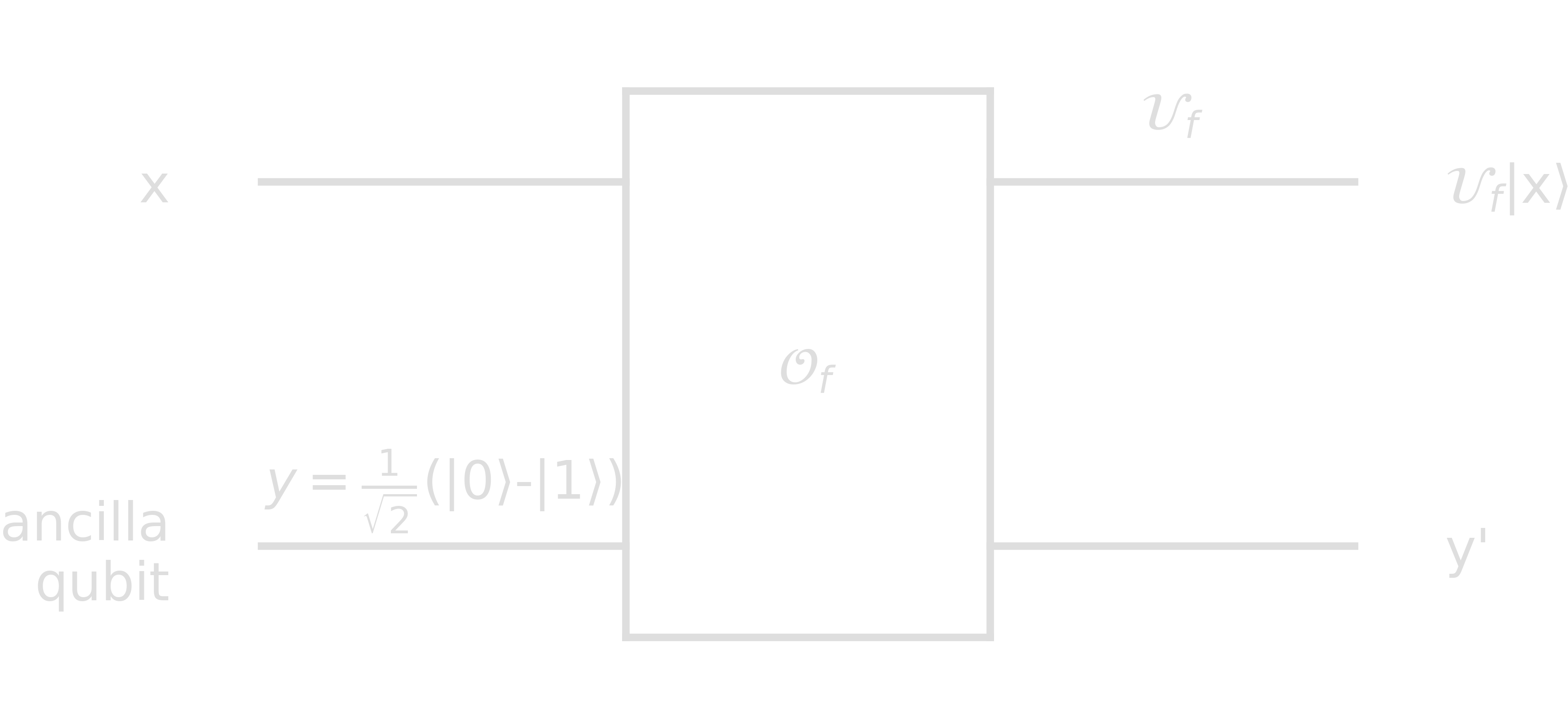
This is independent of \(\ket{y}\), and therefore \(\mathcal{U}_f\): phase oracle performs the map \(\mathcal{U}_f\ket{x} = (-1)^{f(x)}\ket{x}\).
In any case, neither classically nor in a quantum computation, can we find (or tabulate) \(f: {0, 1} \rightarrow {0, 1}\) with a single call. There is however the possibility to find some property of \(f\) with a single query using quantum computation. More specifically, we can find the product \(f(0)f(1)\) or whether \(f(0)=f(1)\). This is what the Deutsch-Jozsa algorithm solves.
Hadamard on n qubits
Recall that
\[\begin{align} H\ket{0} &= \ket{+} = \frasq(\ket{0}+\ket{1})\\ H\ket{1} &= \ket{-} = \frasq(\ket{0}-\ket{1}). \end{align}\]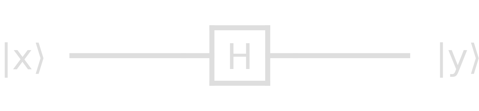
We can reformulate the action of the Hadamard operator to the state \(x \in {0, 1}\) the following way
\[\begin{align} H\ket{x} = \ket{y} &= \frasq(\ket{0}+(-1)^{x}\ket{1}) = \frasq ((-1)^{0\cdot x}\ket{0} + (-1)^{1\cdot x}\ket{1}) \\ &= \frasq \sum_{k\in\{0, 1\}} (-1)^{k\cdot x} \ket{k} \end{align}\]For \(x \in {0, 1}^{n}\), we can generalize this expression easily
\[\begin{align} \ket{y} = H^{\otimes n}\ket{x} = \frasq\sum_{k\in\{0, 1\}^{n}}(-1)^{k\cdot x}ket{k} \end{align}\]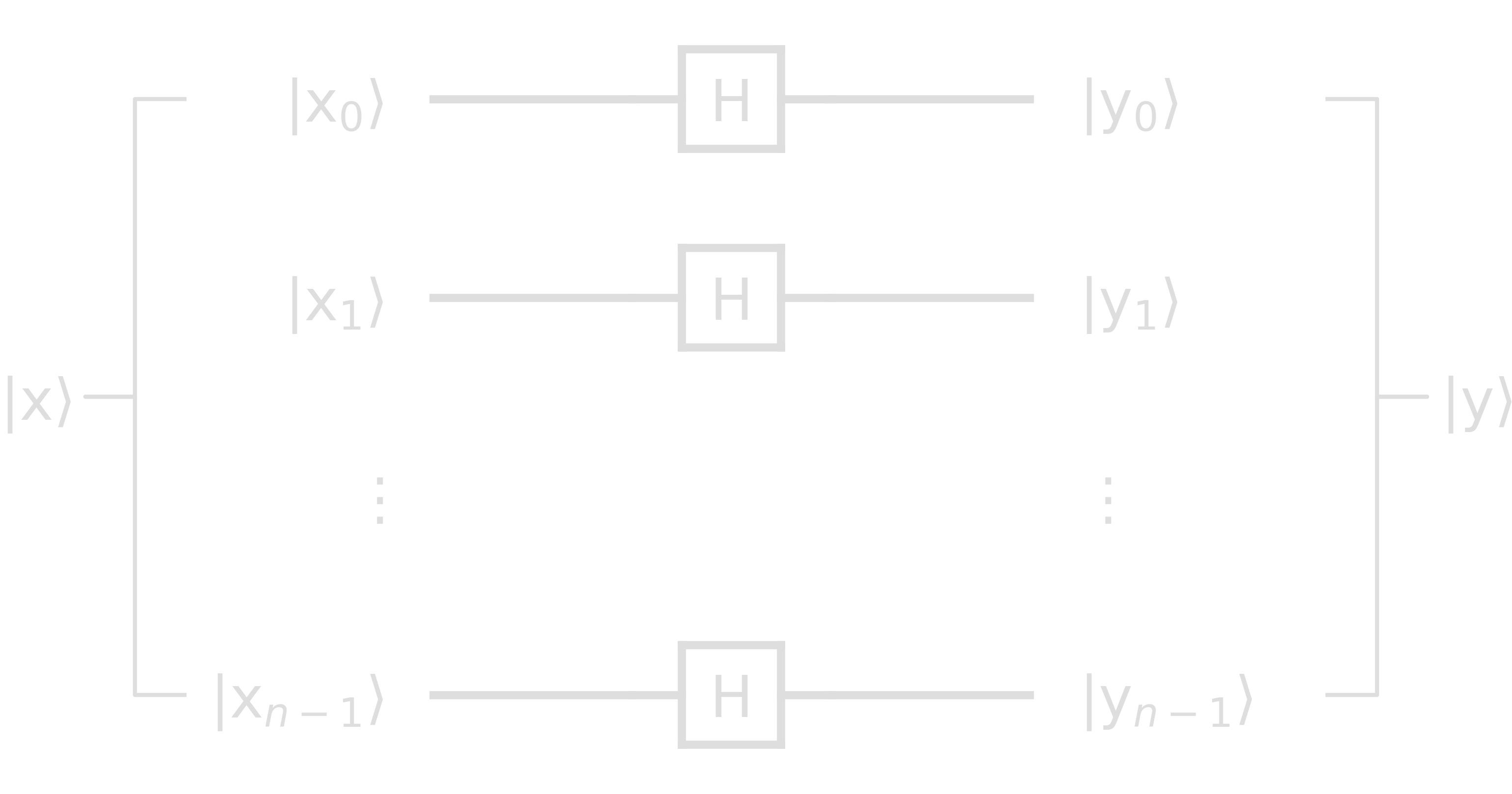
This means that every state \(\ket{y_i}\) is either \(\ket{+}\) or \(\ket{-}\), and \(\ket{y}\) must be a superposition of all possible \(2^n\) bit strings. In the example \(\ket{x}=\ket{01}\)
In this case,
\begin{equation} \ket{y}=\ket{+}\otimes\ket{-}=\frac12(\ket{00}-\ket{01}+\ket{10}-\ket{11}) \end{equation}
Deutsch-Jozsa circuit
Assume, we are given a function \(f: {0, 1}^{n} \rightarrow {0,1}\), realized by an oracle, of which we know that it is either constant (all inputs map to the same output) or balanced (inputs map to 0 and 1 in equal numbers). Our goal is to determine whether \(f\) is constant or balanced.
In the classical approach, we need to ask the oracle at least twice in order to reach a solution, but if we get the same output, we need to ask at least once more… with at most \(\frac{N}{2}+1=2^{n-1}+1\) queries, we are guaranteed to find a solution (\(n\): number of input bits, \(N=2^{n}\): number of realizable bit strings). For example, there are \(2^{n}\) ways to throw a coin.
In the quantum solution only a single query is required. The following is the Deutsch-Jozsa circuit
Claim: If the outcome \(y\) in the DJ circuit (depicted above) equals the bit string \(0^{\otimes n}\), then \(f\) is constant, otherwise it is balanced.
Proof: Let us check the state after every step \(\ket{\psi_0}\), \(\ket{\psi_1}\), \(\ket{\psi_2}\), and \(\ket{\psi_3}\).
\[\begin{align} \ket{\psi_0} &= \ket{00...0} = \ket{0}^{\otimes n}\\ \ket{\psi_1} &= H^{\otimes}\cdot\ket{\psi_0} = \frac{1}{\sqrt{2^{n}}}\sum_{x\in\{0,1\}^{n}}(-1)^{x\cdot\psi_0}\ket{x} = \frac{1}{\sqrt{2^{n}}}\sum_{x\in\{0,1\}^{n}}\ket{x}\\ \ket{\psi_2} &= \mathcal{U}_f\cdot\ket{\psi_1} = \frac{1}{\sqrt{2^{n}}}\sum_{x\in\{0,1\}^{n}}\mathcal{U}_f\ket{x} = \frac{1}{\sqrt{2^{n}}}\sum_{x\in\{0,1\}^{n}}(-1)^{f(x)}\ket{x}\\ \ket{\psi_3} &= H^{\otimes}\cdot\ket{\psi_2} = \frac{1}{\sqrt{2^{n}}}\sum_{x\in\{0,1\}^{n}}(-1)^{f(x)}H^{\otimes}\cdot\ket{x} = \frac{1}{2^{n}}\sum_{x\in\{0,1\}^{n}}(-1)^{f(x)}\sum_{k\in\{0,1\}^{n}}(-1)^{k\cdot x}\cdot\ket{k}\\ &= \sum_{k\in\{0,1\}^{n}}\left[ \frac{1}{2^{n}}\sum_{x\in\{0,1\}^{n}}(-1)^{f(x)+k\cdot x} \right] \ket{k} := \sum_{k\in\{0,1\}^{n}}c_k\ket{k} \end{align}\]The probability to measure the zero string \(\ket{00…0}\) is
\[\begin{align} P[y=0^{\otimes n}] &= |\braket{0^{\otimes n}}{\psi_3}|^{2} = |\sum_{k\in\{0,1\}^{n}} c_k \braket{0^{\otimes n}}{k}|^{2} = |c_{0^{\otimes n}}|^{2}\\ &= |\frac{1}{2^{n}} \sum_{x\in\{0,1\}^{n}} (-1)^{f(x)}|^{2}\\ &= \left\{ \begin{array}{ll} 1 & \mbox{if } f\ \mbox{is constant} \\ 0 & \mbox{if } f\ \mbox{is balanced} \end{array} \right. \end{align}\]\(\square\)
Grover’s algorithm
Grover’s algorithm is designed for “searching an unsorted database” with N=2n elements in \(\mathcal{O}(\sqrt{N})\) time. In this context, “database” can mean a table of function outputs indexed by corresponding inputs. This essentially makes the algorithm a function inversion solver. A classical algorithm needs on average \(\frac{N}{2}=\mathcal{O}(N)\) time to find a solution, as generally we have to check half of all values in order to have a 50% probability to find the target.
Problem statement: Find \(w\), given a (phase) oracle \(\mathcal{U}_f\) with \(\ f: {0, 1}^{n} \rightarrow {0, 1}\)
\[\begin{align} f(x) &= \left\{ \begin{array}{ll} 1 & \mbox{if } x = w \\ 0 & \mbox{else} \end{array} \right.\\ f_0(x) &= \left\{ \begin{array}{ll} 0 & \mbox{if } x = 0^{\otimes n} \\ 1 & \mbox{else} \end{array} \right. \end{align}\]The phase oracle maps \(\mathcal{U}_f\ket{x} = (-1)^{f(x)}\ket{x} = \ket{x}\). Then,
\[\begin{align} &\color{orange}{\mathcal{U}_f}: \left\{ \begin{array}{ll} \ket{w} &\rightarrow -\ket{w} \\ \ket{x} &\rightarrow \ket{x} \quad\forall\ x\neq w \end{array} \right.\\ &\rightarrow\ \mathcal{U}_f = \mathbb{1} - 2\ketbra{w}{w}\\ \\ &\mathcal{U}_{f_0}: \left\{ \begin{array}{ll} \ket{0}^{\otimes n} &\rightarrow \ket{0}^{\otimes n} \\ \ket{x} &\rightarrow -\ket{x} \quad\forall\ x\neq 0^{\otimes n} \end{array} \right.\\ &\rightarrow\ \mathcal{U}_{f_0} = 2\ketbra{0}{0}^{\otimes n} - \mathbb{1} \end{align}\]The quantum circuit for Grover’s algorithm is as follows
Claim: \(y = w\) with high probability.
Proof: Let us define the uniform superposition states
\[\begin{align} \color{turquoise}{\ket{s}} &:= H^{\otimes n} \ket{0}^{\otimes n} = \frac{1}{\sqrt{2^{n}}} \sum_{x\in\{0,1\}^{n}} \ket{x}\\ \end{align}\]and the “diffusion” operator
\[\begin{align} \color{hotpink}{V} &:= H^{\otimes n}\cdot\mathcal{U}_{f_0}\cdot H^{\otimes n} = H^{\otimes n}\cdot 2\ketbra{0}{0}^{\otimes n}\cdot H^{\otimes n} - H^{\otimes n}\cdot H^{\otimes n} = 2\ketbra{s}{s} - \mathbb{1} \end{align}\]With these definitions, Grover’s algorithm carries out the operation \((V\cdot\mathcal{U}_f)^{r}\) on the state \(\ket{s}\). Corresponding to this, there is a geometric respresentation which nicely explains the mechanism behind this operation: Let \(\Sigma\) be the plane spanned by \(\ket{s}\) and \(\ket{w}\) and let \(\ket{w^\bot}\) be the state orthogonal to \(\ket{w}\) in \(\Sigma\).
\[\begin{align} &\ket{w^{\bot}} := \frac{1}{\sqrt{2^n-1}} \sum_{x\neq w}\ket{x}\\ &\Rightarrow \ket{s} = \sqrt{\frac{2^n-1}{2^n}} \ket{w^\bot} + \frac{1}{\sqrt{2^n}} \ket{w} =: \cos{\frac{\theta}{2}}\ket{w^\bot} + \sin{\frac{\theta}{2}}\ket{w} \end{align}\]
Protocol:
- Prepare \(\color{turquoise}{\ket{s}}\)
- Apply \(\color{orange}{\mathcal{U}_f=\mathbb{1}-2\ketbra{w}{w}}\)
- Apply \(\color{hotpink}{V=2\ketbra{s}{s}-\mathbb{1}}\)
\(V\cdot\mathcal{U}_f\) corresponds to a rotation by an angle \(\theta\). After r applications of 2 and 3, the state is rotated by \(r\cdot\theta\). However, the rotation only ends up at the target state \(\ket{w}\), if the right number of repetitions is chosen. Therefore, choose r, such that
\begin{equation} r\cdot\theta+\frac{\theta}{2} \approx \frac{\pi}{2}. \end{equation}
This means
\begin{equation} r = \frac{\pi}{2\theta} - \frac12 = \frac{\pi}{4\arcsin{\frac{1}{\sqrt{2^n}}}} - \frac12 \approx \frac{\pi}{4}\sqrt{2^n} = \mathcal{O}(\sqrt{N}) \end{equation}
After r calls to the oracle, the final measurement will result in state \(\ket{w}\) with minimal probability of deviation.
\begin{equation} P(w) \geq 1 - \sin^2{\frac{\theta}{2}} = 1 - \frac{1}{2^n} \end{equation}
\(\square\)
Amplitude amplification
The general idea behind Grover’s algorithm is amplitude amplification. Let us have a look at the amplitudes at each step in Grover’s algorithm:
Step 1. \(\ket{s} := H^{\otimes n}\ket{0}^{\otimes n}\)
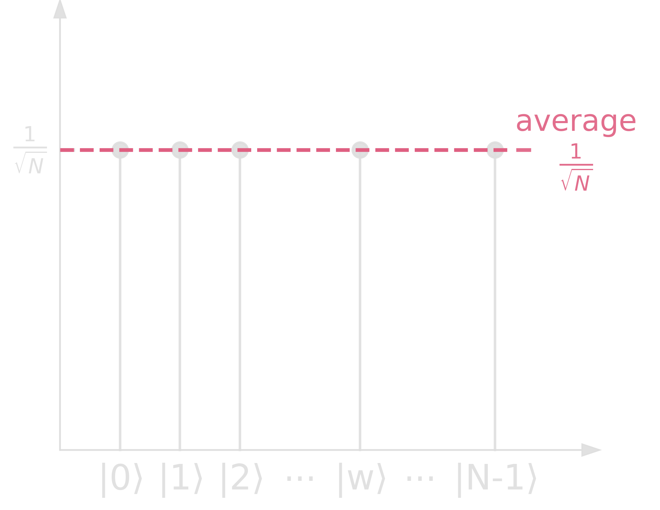
Step 2. \(\mathcal{U}_f\cdot\ket{s} = (2\ketbra{s}{s}-\mathbb{1})\ket{s}\): flip amplitude of \(\ket{w}\)
Step 3. \(V\cdot\mathcal{U}_f\cdot\ket{s} = (2\ketbra{s}{s}-\mathbb{1})\cdot\mathcal{U}_f\cdot\ket{s}\): reflect amplitudes about the average amplitude
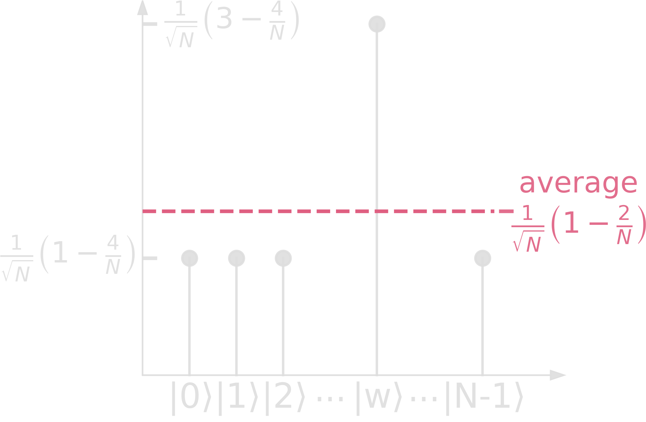
By repeating steps 2 and 3, the amplitude of \(\ket{w}\) will increase further, making the process an amplitude amplification!
As for \(\ket{\psi} := \sum_i{\alpha_i\ket{i}}\), \(V\cdot\ket{\psi}\) yields:
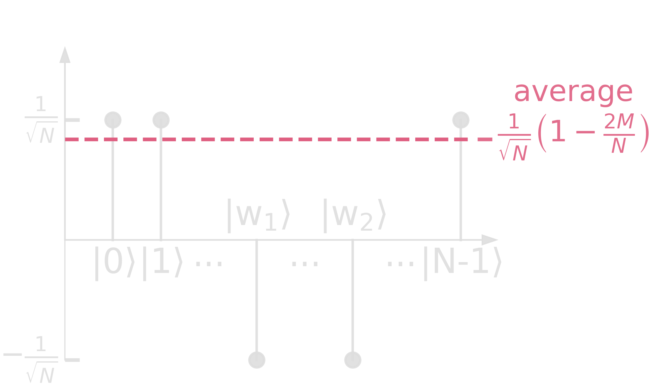
\[\begin{align} (2\ketbra{s}{s}-\mathbb{1})\cdot\ket{\psi} &= \frac{2}{N}\cdot\sum_j{\ket{j}}\cdot\sum_k{\bra{k}}\cdot\sum_i{\alpha_i\ket{i}} - \sum_i{\alpha_i\ket{i}}\\ &= 2\cdot\frac{\sum_k{\alpha_k}}{N}\cdot\sum_j{\ket{j}}-\sum_j{\alpha_j\ket{j}}\\ &= \sum_j{(2\cdot\langle\alpha\rangle-\alpha_j)\ket{j}} \end{align}\]The term \((2\cdot\langle\alpha\rangle-\alpha_j)\) is the reflection of \(\alpha_j\) about the average \(\langle\alpha\rangle\). If \(\alpha_j=\langle\alpha\rangle + \Delta\), then \(\alpha_j’=2\langle\alpha\rangle-\alpha_j = \langle\alpha\rangle-\Delta\).
Multiple marked elements
When we have M marked elements \(w_i\), we define the winning state as
\[\begin{align} \ket{w} &:= \frac{1}{\sqrt{M}} \sum_{i=1}^{M}{\ket{w_i}}\\ \ket{w^\bot} &= \frac{1}{\sqrt{N-M}}\cdot\sum_{x\notin\{w_1,\dots w_\mu\}}\ket{x}\\ &\Rightarrow \ket{s} = \frac{\sqrt{N-M}}{\sqrt{N}}\cdot\ket{w^\bot} + \sqrt{\frac{M}{N}}\cdot\ket{w} =: \cos{\frac{\theta}{2}}\ket{w^\bot}+\sin{\frac{\theta}{2}}\ket{w}\\ &\rightarrow \sin{\frac{\theta}{2}} = \sqrt{\frac{M}{N}} \end{align}\]This means the angle becomes larger!
\begin{equation} r = \frac{\pi}{4\arcsin{\sqrt{\frac{M}{N}}}} - \frac12 = \mathcal{O}\left(\sqrt{\frac{N}{M}}\right) \end{equation}
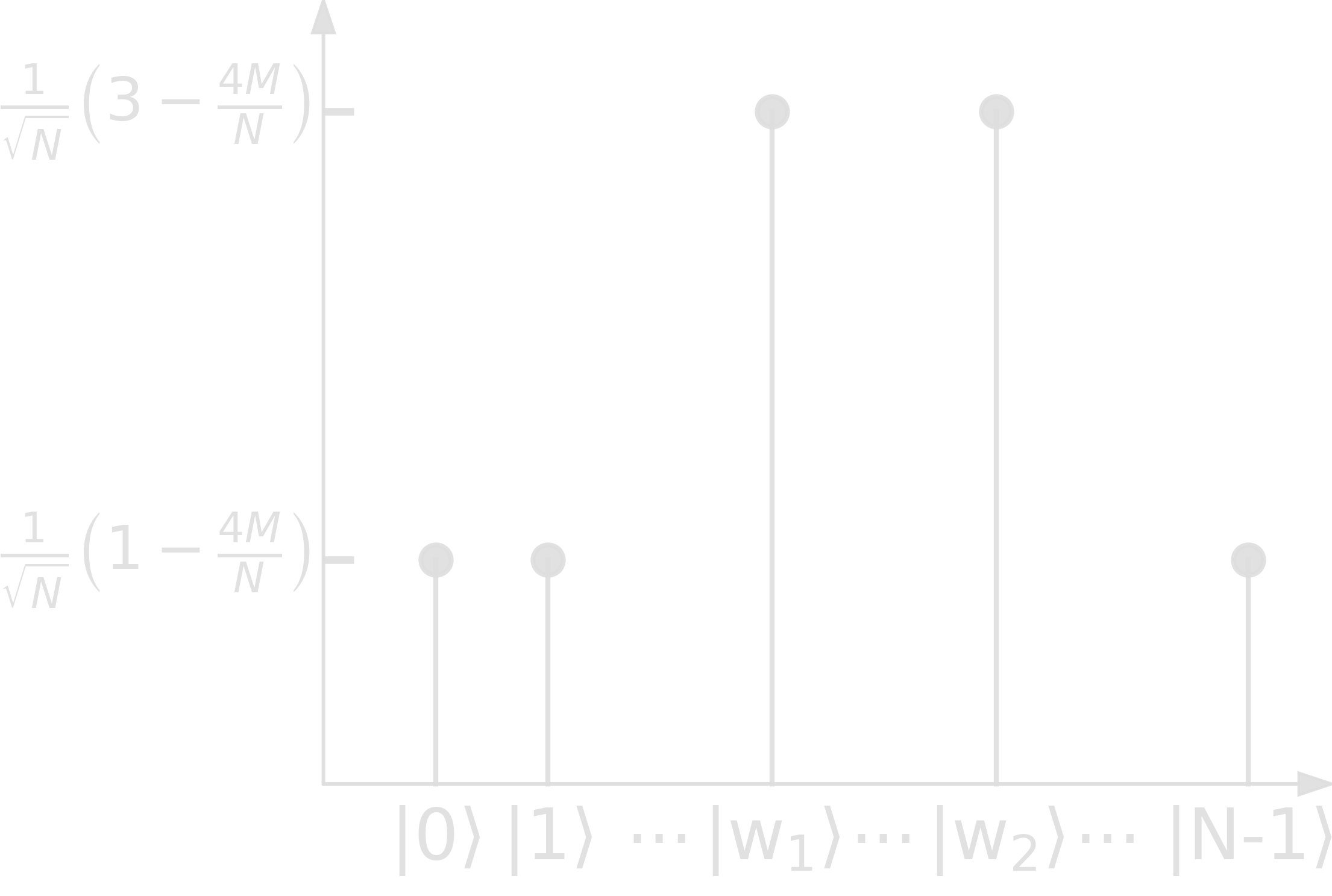
The speed-up can also be seen when looking at amplitudes!
Step 1.
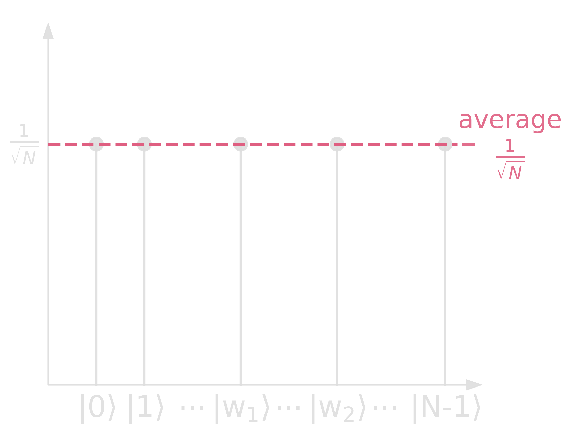
Step 2.
Step 3. Results in faster amplitude amplification!
Shor’s algorithm
Shor’s algorithm is probably the most famous quantum algorithm. It solves the problem of efficient integer factorization, which, on an ideal quantum computer, can be used to break cryptographic ciphers.
Recap
Summary: Qubits and quantum states
\[\begin{array}{ll} \ket{0} = \cvec{0 \\ 1} & \ket{1} = \cvec{1 \\ 0} \\ H = \frasq\cvec{1&1 \\ 1&-1} & X = \cvec{0&1 \\ 1&0} \\ \ket{\psi} = a \ket{0} + b \ket{1} & \\ \braket{0}{\psi} = a & \braket{1}{\psi} = b \\ P(0) = |a|^2 & P(1) = |b|^2 \\ |a|^2 + |b|^2 = 1 & \\ \end{array}\]Operations on quantum states need to preserve norm to 1, i.e. quantum operators are unitary
\[\begin{align} \rightarrow\quad & U^\dagger = U^{-1} \\ & U^\dagger U = UU^\dagger = \mathbb{1} \\ \rightarrow\quad & |\det{U}| = 1 \end{align}\]For single qubits, unitary gates can be thought of as rotation on the surface of the Bloch sphere.
Eigenvalues and eigenvectors of unitary matrices are special
1 )
\begin{equation} U\ket{x} = \lambda_x\ket{x} \quad\Rightarrow\quad \bra{x}U^\dagger = \bra{x}\lambda^\ast_x \end{equation}
\[\begin{align} &\braket{x}{x} = 1 = \bra{x}U^\dagger U\ket{x} = \bra{x}\lambda^\ast_x\lambda_x\ket{x} = |\lambda_x|^2 \\ &\Rightarrow\quad |\lambda_x|^2 = 1 \\ &\Rightarrow\quad \lambda_x = e^{i\theta_x} \\ \end{align}\]This means the eigenvalues of \(U\) are of the form \(e^{i\theta}\).
2 )
\[\begin{align} &U\ket{x} = \lambda_x\ket{x} \\ &U\ket{y} = \lambda_y\ket{y} \end{align}\]if \(\lambda_x\neq\lambda_y\), then
\[\begin{align} &\braket{x}{y} = \bra{x}U^\dagger U\ket{x} = \lambda^\ast_x\lambda_y \braket{x}{y} \\ &\Rightarrow\quad \braket{x}{y}(1-\lambda^\ast_x\lambda_y) = 0 \\ &\Rightarrow\quad \braket{x}{y}(\lambda_x-\lambda_y) = 0 \end{align}\]Quantum algorithms use a sequence of these unitary operators to solve problems:
- Deutsch-Jozsa algorithm: constant vs. balanced function in one shot
- Grover’s algorithm: unstructed search in N items with \(\mathcal{O}(\sqrt{N})\)
Preliminaries
Factoring a number \(N=p\cdot q\) where \(p\) and \(q\) are primes and large is a classically difficult problem. Modular arithmetic is important to understand when trying to solve number factorization. For instance,
\[\begin{align} 5 &\div 3 = \begin{array}{ll} &\mbox{ quotient } 1\\ &\mbox{ remainder } 2 \end{array}\\ 5 &\equiv 2\ (\mathrm{mod}\ 3) \end{align}\]\begin{array}{llllllllllll}
& x & 1 & 2 & 3 & 4 & 5 & 6 & 7 & 8 & 9 &
x & \equiv & 1 & 2 & 0 & 1 & 2 & 0 & 1 & 2 & 0 & (\mathrm{mod}\ 3)
\end{array}
Notice that for \(x\equiv 0\ (\mathrm{mod}\ 3)\), x is a multiple of 3, for \(x\equiv 1\ (\mathrm{mod}\ 3)\), x is \(1+\) some multiple of 3. Generally, for
\begin{equation} x\equiv y\ (\mathrm{mod}\ N) \quad\Rightarrow\quad x=Nk+y \mbox{ for } k\in\mathbb{Z} \end{equation}
Note that this modular function is periodic, meaning
\begin{equation} x \equiv y\ (\mathrm{mod}\ N)\quad\Rightarrow\quad y\in{0, 1, 2, \ldots, N} \end{equation}
Shor’s algorithm consists of solutions of multiple subproblems. The problem of finding the period of a given periodic function is certainly amongst the most important ones. More specifically, we look for a period \(p\) of a function \(f\) such that
\begin{equation} f(x) = f(y)\ \mbox{ for } x\neq y \mbox{ iff } |x-y|=kp \mbox{ with } k\in\mathbb{Z} \end{equation}
- A very easy example would be
- A slightly harder one
Classically, this problem can be solved in \(\mathcal{O}(\exp{cn^{\frac13}(\log{n})^\frac23})\) with \(p\) consisting of \(n\) bits. The complexity of quantum Shor’s algorithm is \(\mathcal{O}(n^2(\log{n})(\log{\log{n}}))\) which is a little faster than \(\mathcal{O}(n^3)\).
The period-finding algorithm is at the heart of Shor’s algorithm. Using quantum superposition, we would ideally evaluate the function in question simultaneously at all points. Unfortunately, the no-cloning theorem prohibits a repeated measurement on the same superposition, so we need a trick that extracts the right solution from it with high probability. That trick is the quantum Fourier transform.
Thus, Shor’s algorithm consists of three implementations:
- Creation of a superposition state (using Hadamard gates or quantum Fourier transform)
- modular exponentiation to find co-primes of the target number \(N=p\cdot q\) using Euler’s totient theorem
- quantum phase estimation/quantum Fourier transform to extract the period of the modular function
Quantum Fourier transformation
Quantum Fourier transform (QFT) is effectively a change of basis from the computational to a Fourier basis. For instance, states in the computational basis are \(\ket{0}\) and \(\ket{1}\), in the Fourier basis \(\ket{+}\) and \(\ket{-}\). For a single qubit, the Hadamard transformation achieves exactly that, but for multi-qubit states QFT takes that tranformation role.
Notice that we go from a basis on the two poles of the Bloch sphere to a basis on the equatorial plane.
With \(n\) qubits there are \(2^n\) basis states. Let us define \(N=2^n\). Then the Fourier basis is defined as
\begin{equation} \ket{\tilde{x}} := \mathrm{QFT}{\ket{x}} = \frac{1}{\sqrt{N}} \sum_{y=0}^{N-1}{e^{\frac{2\pi ixy}{N}}\ket{y}} \end{equation}
In the case of 1 qubit, i.e. \(N=2\), this is as expected
\[\begin{align} \ket{\tilde{0}} &= \frasq\sum_{y=0}^{1}{e^{\frac{2\pi i(0)y}{2}}\ket{y}} = \frasq\sum_{y=0}^{1}{\ket{y}} \\ &= \frasq\left(\ket{0}+\ket{1}\right) \\ \ket{\tilde{1}} &= \frasq\sum_{y=0}^{1}{e^{\frac{2\pi i(1)y}{2}}\ket{y}} = \frasq\left(e^{\frac{2\pi i(0)}{2}}\ket{0}+e^{\frac{2\pi i(1)}{2}}\ket{1}\right) \\ &= \frasq\left(\ket{0}+(-1)\ket{1}\right) = \frasq\left(\ket{0}-\ket{1}\right) \\ \end{align}\]Note that we here we use the binary notation, e. g. \(\ket{4} = \ket{100}\).
We can rewrite the transform as
\[\begin{align} \ket{\tilde{x}} &= \frac{1}{\sqrt{N}}\sum_{y=0}^{N-1}e^{\frac{2\pi ixy}{N}}\ket{y}\\ &= \frac{1}{\sqrt{N}}\sum_{y_1=0}^{1}\sum_{y_2=0}^{1}\cdots\sum_{y_n=0}^{1}e^{\frac{2\pi ix}{N}\sum_{k=1}^{n}y_{k}2^{n-k}}\ket{y_k}\\ &= \frac{1}{\sqrt{N}}\sum_{y_1,y_2,\ldots y_n}\bigotimes_{k=1}^{n}e^{\frac{2\pi ix}{N}2^{n-k}y_{k}}\ket{y_k}\\ &= \frac{1}{\sqrt{N}}\bigotimes_{k=1}^{n}\left[\ket{0}+e^{\frac{2\pi ix}{N}2^{n-k}}\ket{1}\right]\\ &= \frac{1}{\sqrt{N}}\bigotimes_{k=1}^{N}\left[\ket{0}+e^{2\pi ix\,2^{-k}}\ket{1}\right]\\ %&= \frac{1}{\sqrt{N}}\sum_{y=0}^{N-1}e^{2\pi ix\sum_{k=1}^{n}\frac{y_k}{2^k}}\ket{y_1y_2\cdots y_n} \end{align}\]for which the \(k=1\) term is
\begin{equation} \ket{0} + e^{2\pi i \frac{x}{2}}\ket{1} \end{equation}
and the \(k=2\) term is
\begin{equation} \ket{0} + e^{2\pi i \frac{x}{4}}\ket{1} \end{equation}
Notice that a division by 2 shifts the binary number to the right and fills it with “0”s at the left
\[\begin{align} x &= \left[x_1\ x_2\ x_3\ x_4 \cdots x_n\right]\\ \frac{x}{2} &= \left[0\;\ x_1\ x_2\ x_3 \cdots x_{n-1}\right]\\ \frac{x}{4} &= \left[0\;\ 0\;\ x_1\ x_2 \cdots x_{n-2}\right]\\ \end{align}\]Thus, the mapping of the QFT finally takes the form
\begin{equation}\label{eq:qft} \ket{x} = \ket{x_1x_2\cdots x_n} \rightarrow \ket{\tilde{x}} = \frac{1}{\sqrt{N}}\left(\ket{0}+e^{2\pi i\frac{x}{2}}\ket{1}\right)\otimes\left(\ket{0}+e^{2\pi i\frac{x}{4}}\ket{1}\right)\otimes\cdots\otimes\left(\ket{0}+e^{2\pi i\frac{x}{2^n}}\ket{1}\right) \end{equation}
Each qubit transforms from \(\ket{x_k}\) to \(\ket{0}+e^{2\pi i\frac{x}{2^k}}\ket{1}\).
For example, \(n=3\) qubits (\(N=2^3=8\)):
\[\begin{align} \ket{x} &= \ket{5}\\ \mathrm{QFT}\ket{x} &= \frac{1}{\sqrt{8}}\left(\ket{0}+e^{2\pi i\frac{5}{2}}\ket{1}\right)\otimes\left(\ket{0}+e^{2\pi i\frac{5}{4}}\ket{1}\right)\otimes\left(\ket{0}+e^{2\pi i\frac{5}{8}}\ket{1}\right)\\ \end{align}\]Notice that this represents a rotation around the y-axis on the unit sphere, because
\[\begin{align} 2\pi i\left(\frac{5}{2}\right) &= 2\pi i\left(\frac{2^2}{2}+\frac12\right)\\ &= 2\pi i\left(2+\frac12\right) \end{align}\]and since \(e^{2\pi iz}=1\ \forall\,z\in\mathbb{Z}\)
\begin{equation} e^{2\pi i\left(\frac52\right)} = e^{2\pi i\left(2+\frac12\right)} = e^{2\pi i\left(\frac12\right)} = e^{i\pi} = -1 \end{equation}
We can make two observations about the QFT transform:
- \(\ket{\tilde{x}}\) contains terms like
- phase is qubit-dependent and more components add up with more “1”s
The construction of the QFT circuit makes use of two ingredients:
- the Hadamard gate
- the UROTk gate, a two-qubit controlled rotation gate that requires target and control qubits to be adjacent. It applies a phase of \(e^{2\pi i/2^k}\).
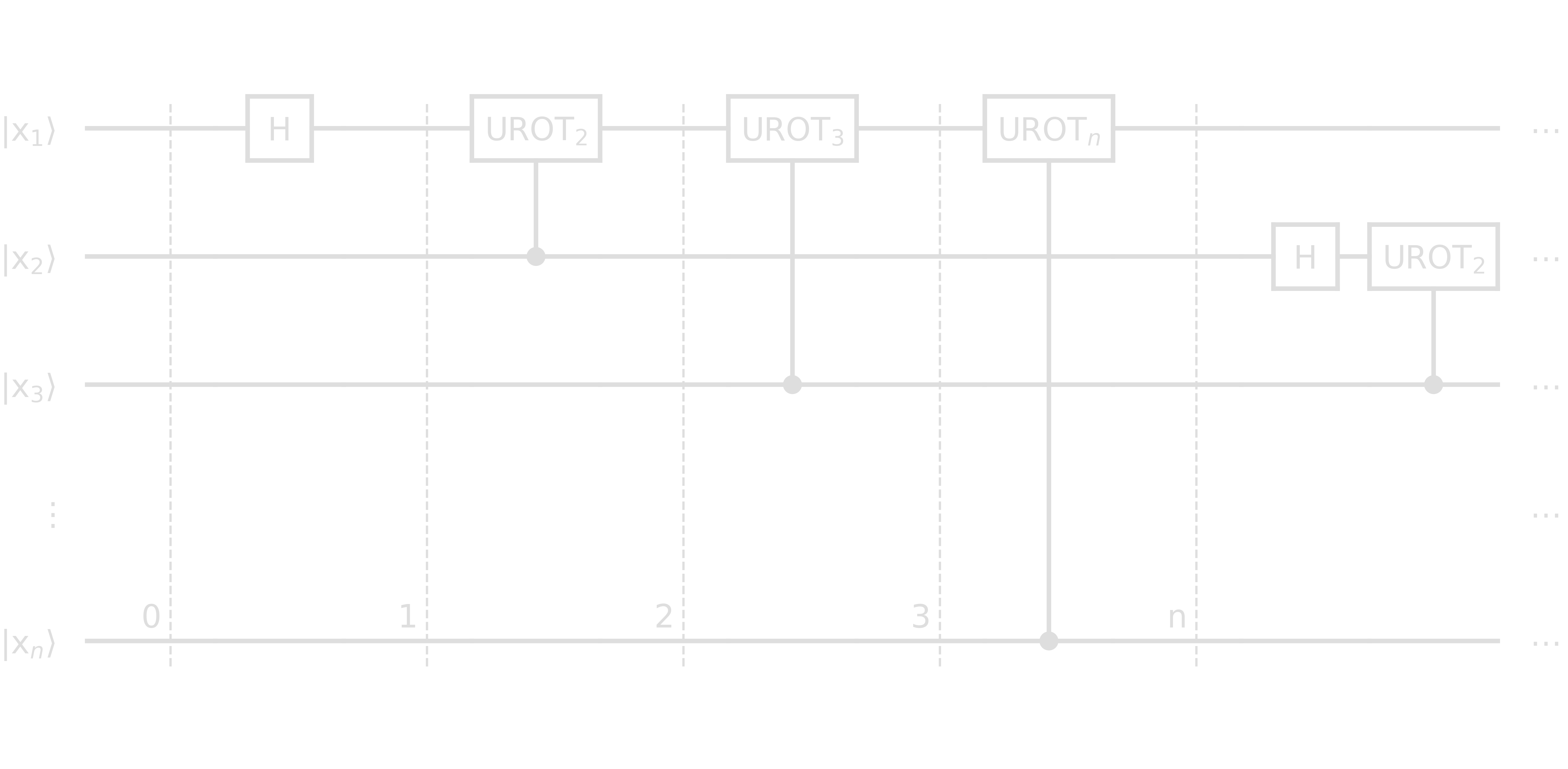
- Step 0: \(\ket{x} = \ket{x_1\ x_2\cdots x_n}\)
- Step 1: \(\left[\ket{0}+e^{\frac{2\pi i}{2}x_1}\ket{1}\right]\otimes\ket{x_2\cdots x_n}\)
- Step 2: \(\left[\ket{0}+e^{\frac{2\pi i}{2^2}x_2}e^{\frac{2\pi i}{2}x_1}\ket{1}\right]\otimes\ket{x_2\cdots x_n}\)
- Step 3: \(\left[\ket{0}+e^{\frac{2\pi i}{2^3}x_3}e^{\frac{2\pi i}{2^2}x_2}e^{\frac{2\pi i}{2}x_1}\ket{1}\right]\otimes\ket{x_2\cdots x_n}\)
- Stepn: \(\left[\ket{0}+e^{\frac{2\pi i}{2^n}x_n}\cdots e^{\frac{2\pi i}{2}x_1}\ket{1}\right]\otimes\ket{x_2\cdots x_n}=\left[\ket{0}+\exp\left({2\pi i\left[\frac{x_n}{2^n}+\cdots +\frac{x_1}{2^1}\right]}\right)\ket{1}\right]\otimes\ket{x_2\cdots x_n}\)
Recall that
\[\begin{align} x &= 2^{n-1}x_1 + 2^{n-2}x_2 + \cdots + 2^{0}x_n \\ &\Rightarrow\quad \frac{x_n}{2^n} + \cdots + \frac{x_1}{2^1} = \frac{x}{2^n} \\ &\Rightarrow\quad \exp\left({2\pi i\left[\frac{x_n}{2^n}+\cdots +\frac{x_1}{2^1}\right]}\right) = \exp\left[2\pi i\frac{x}{2^n}\right] \end{align}\]Therefore, after n steps the qubit state is
\begin{equation} \left[\ket{0}+e^{2\pi i\frac{x}{2^n}}\ket{1}\right]\otimes\ket{x_2\cdots x_n} \end{equation}
This can be repeated for the qubits \(x_2\) to \(x_n\) and we end up with Equation (\ref{eq:qft}), with the caveat that the order of the qubits is reversed in the output state.
Quantum Phase Estimation
A unitary matrices such as transformations of quantum gates have eigenvalues of the form \(e^{i\theta}\) and eigenvectors which form an orthonormal basis
\begin{equation} U\ket{\psi} = e^{i\theta_\psi}\ket{\psi} \end{equation}
Quantum phase estimation enables us to find \(\theta_\psi\) given the ability to prepare \(\psi\). QPE is an important subroutine in other quantum algorithms such as Shor’s algorithm or the quantum algorithm for linear systems of equations.
It uses phase kickback to write the phase of the U-gate (in the Fourier basis) to the \(n\) qubits in the counting register. Phase kickback is where the eigenvalue added by a gate to a qubit is ‘kicked back’ into a different qubit via a controlled operation. Recall from the QFT transformation that the upper-most qubit performs a full rotation when counting from \(0\) to \(2^n\). In order to count to a number x between \(0\) and \(2^n\), we rotate this qubit by \(\frac{x}{2^n}\), the next by \(\frac{2x}{2^n}\), then \(\frac{4x}{2^n}\) etc.
When a qubit is used to control the U-gate, it is rotated by a phase proportional to \(e^{i\theta_\psi}\). If the rotation is repeated an appropriate amount of times, it is encoded in the counting register as a number between \(0\) and \(2^{n}\) (where \(n\) is the size of the counting register) in the Fourier basis. A simple inverse QFT transformation converts this phase into the computational basis where it can be measured.
The QPE circuit consists of Hadamard gates and controlled U gates.
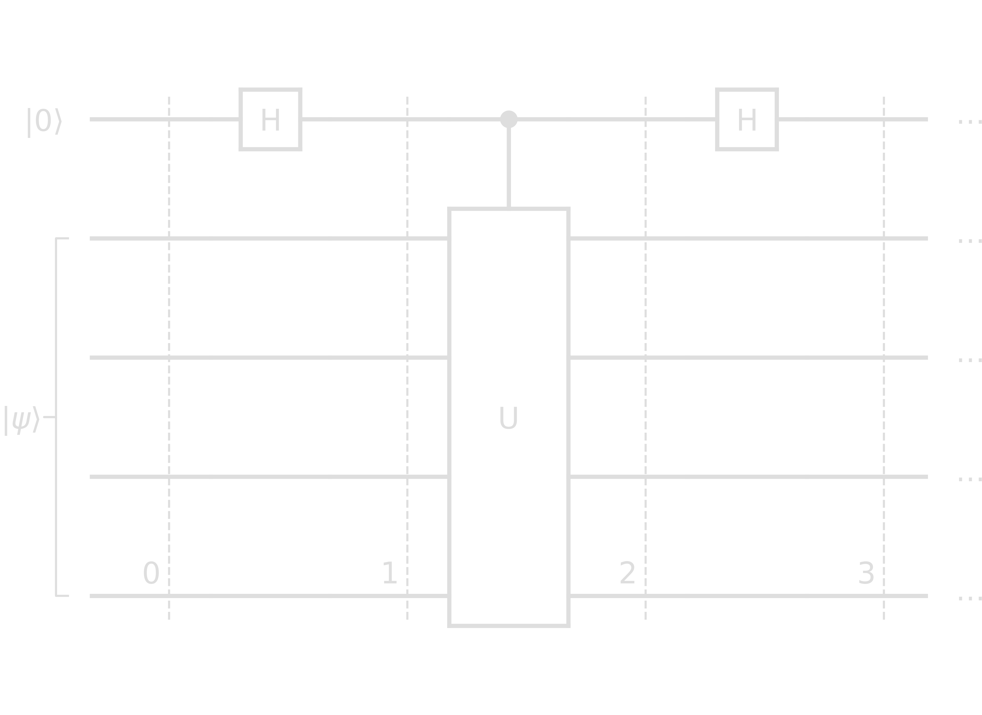
- Step 0: \(\ket{0}\ket{\psi}\)
- Step 1: \((\ket{0}\ket{\psi} + \ket{1}\ket{\psi})/\sqrt{2}\)
- Step 2: \((\ket{0}\ket{\psi} + \ket{1}e^{i\theta_\psi}\ket{\psi})/\sqrt{2}\)
- Step 3: \(\left[(\ket{0}+\ket{1})\ket{\psi}+e^{i\theta_\psi}(\ket{0}-\ket{1})\ket{\psi}\right]/2 = \left[\ket{0}(1+e^{i\theta_\psi})+\ket{1}(1-e^{i\theta_\psi})\right]\ket{\psi}/2\)
Measurement on qubit \(\ket{0}\) gives probabilities of
\[\begin{align} &\left|\frac{1+e^{i\theta_\psi}}{2}\right|\quad\rightarrow\quad 0\\ &\left|\frac{1-e^{i\theta_\psi}}{2}\right|\quad\rightarrow\quad 1 \end{align}\]These probabilities are almost 50/50, but with a small shift. For \(\theta_\psi > 0\)
\[\begin{align} \mathrm{Prob}[0] &= \cos^2{\frac{\theta_\psi}{2}}\\ \mathrm{Prob}[1] &= \sin^2{\frac{\theta_\psi}{2}} \end{align}\]For a precise measurement of \(\theta_\psi\) using this bit of information, a lot of measurements are needed. Therefore, we use multiple qubits to measure the phase
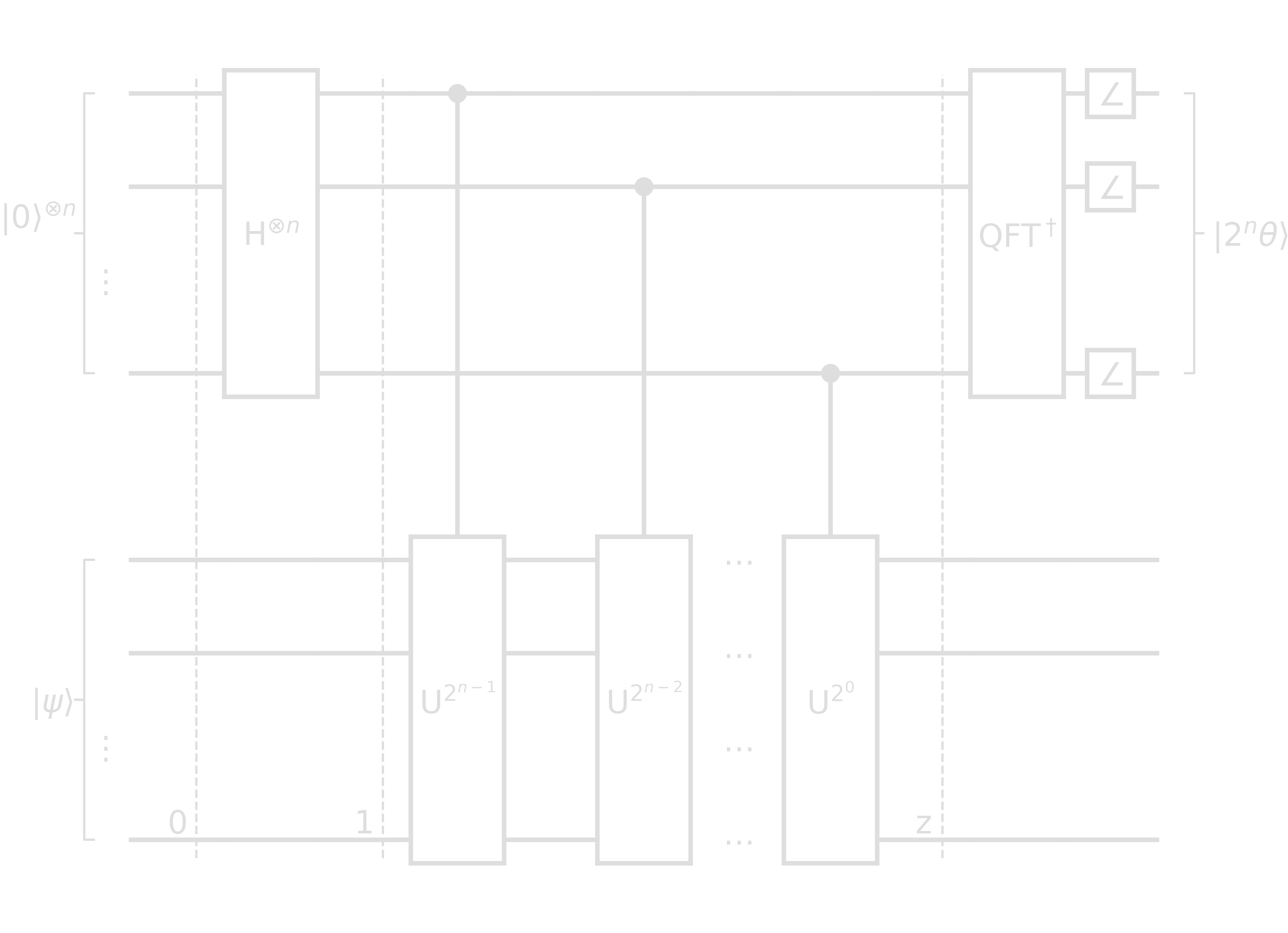
Note that
\[\begin{align} U^{2^x}\ket{\psi} &= U^{2^x-1}U\ket{\psi}\\ &= U^{2^x-1}e^{i\theta_\psi}\ket{\psi}\\ &\quad\vdots \\ &= e^{i\theta_\psi 2^x}\ket{\psi} \end{align}\]- Step 0: \(\ket{0}^{\otimes n}\ket{\psi}\)
- Step 1: \((\ket{0}+\ket{1})^{\otimes n}/\sqrt{2}^n \ket{\psi}\)
- Step z: \(\left(\frasq\right)^{n}\left(\ket{0}+e^{i\theta_\psi2^{n-1}}\ket{1}\right)\otimes\left(\ket{0}+e^{i\theta_\psi2^{n-2}}\ket{1}\right)\otimes\cdots\otimes\left(\ket{0}+e^{i\theta_\psi2^{0}}\ket{1}\right)\)
In comparison to QFT:
\begin{equation} \ket{\tilde{x}} = \left(\frasq\right)^{n}\left(\ket{0}+e^{\frac{2\pi ix}{2^1}}\ket{1}\right)\otimes\left(\ket{0}+e^{\frac{2\pi ix}{2^2}}\ket{1}\right)\otimes\cdots\otimes\left(\ket{0}+e^{\frac{2\pi ix}{2^n}}\ket{1}\right) \end{equation}
QPE and QFT have the same form, but \(\theta_\psi \rightarrow 2\pi\frac{\theta_\psi}{2^n}\). Thus, we can apply an inverse QFT transform to the qubits in the counting register after step z. A measurement should yield \(\frac{1}{2\pi}2^n\theta\).
Shor’s circuit
Shor’s complete algorithm goes as follows
- Pick “a” coprime, i.e. \(\mathrm{gcd}(a, N)=1\), with \(N=p\cdot q\).
- Find “r” the order, i.e. the smallest r s.t. \(a^r \equiv 1\ (\mathrm{mod}\ N)\), of the function \(a^r\ (\mathrm{mod}\ N)\).
-
- if r is even
- \(x \equiv a^{r/2}\ (\mathrm{mod}\ N)\)
- if \(x+1 \not\equiv 0\ (\mathrm{mod}\ N)\) then
- \({p, q} = {\mathrm{gcd}(x+1, N), \mathrm{gcd}(x-1, N)}\)
- otherwise pick another “a” and return to 2.
- if r is even
Let us work through an example: factoring \(N = 15 = \left[1111\right]\) using 4 bits
- Coprime: pick \(a=13\)
- \(13^x\ (\mathrm{mod}\ 15) = 1, 13, 4, 7, 1, 13, 4, 7\) for \(x=0, 1, 2, 3, 4, 5, 6, 7\)
- Smallest \(r>0\) s.t. \(13^r \equiv 1\ (\mathrm{mod}\ 15)\) is \(r=4\).
- Given r=4
- \(x \equiv 13^{4/2}\ (\mathrm{mod}\ 15) \equiv 4\ (\mathrm{mod}\ 15)\)
- \(x+1 = 5 \not\equiv 0\ (\mathrm{mod}\ 15)\)
- Factorization is \({p, q} = {4-1, 4+1} = {3, 5}\)
The circuit for this problem looks as follows
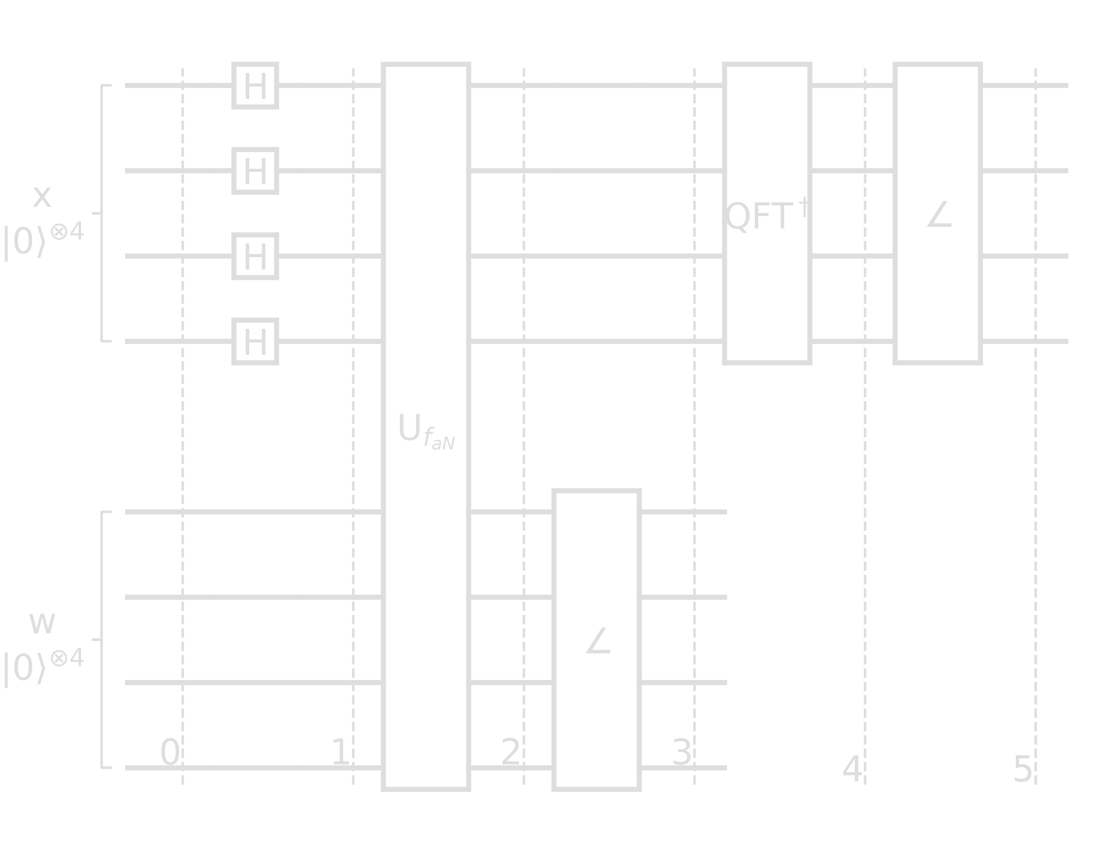
- Step 0: \(\ket{x}\ket{w} = \ket{0}^{\otimes 4}\ket{0}^{\otimes 4}\)
-
Step 1:
\begin{equation} \left[H^{\otimes 4}\ket{0}^{\otimes 4}\right]\ket{0}^{\otimes 4} = \frac14\left[\ket{0}_4+\ket{1}_4+\ket{2}_4+\cdots+\ket{15}_4\right]\ket{0}_4 \end{equation}
- Step 2: \(\begin{align} &\frac14\left[\ket{0}_4\ket{0\oplus 13^0\ (\mathrm{mod}\ 15)}_4 + \ket{1}_4\ket{0\oplus 13^1\ (\mathrm{mod}\ 15)}_4 + \ldots\right]\\ &\mbox{ since } 0\oplus z = z\\ =& \frac14[\ket{0}_4\ket{1}_4 + \ket{1}_4\ket{13}_4 + \ket{2}_4\ket{4}_4 + \ket{3}_4\ket{7}_4 \\ &+\ket{4}_4\ket{1}_4 + \ket{5}_4\ket{13}_4 + \ket{6}_4\ket{4}_4 + \ket{7}_4\ket{7}_4 \\ &+\ket{8}_4\ket{1}_4 + \ket{9}_4\ket{13}_4 + \ket{10}_4\ket{4}_4 + \ket{11}_4\ket{7}_4 \\ &+\ket{12}_4\ket{1}_4 + \ket{13}_4\ket{13}_4 + \ket{14}_4\ket{4}_4 + \ket{15}_4\ket{7}_4 ] \end{align}\)
-
Step 3: after measuring the w register, let’s say we measured 7
\begin{equation} \frac12\left[\ket{3}_4+\ket{7}_4+\ket{11}_4+\ket{15}_4\right]\otimes\ket{7}_4 \end{equation}
- Step 4: apply QFT\(^\dagger\) on the x register \(\begin{align} \mathrm{QFT}\ket{x} = \ket{\tilde{x}} &= \frac{1}{\sqrt{N}}\sum_{y=0}^{N-1}\exp\left({\frac{2\pi i}{N}xy}\right)\ket{y}\\ \mathrm{QFT}^{\dagger}\ket{x} = \ket{x} &= \frac{1}{\sqrt{N}}\sum_{y=0}^{N-1}\exp\left({-\frac{2\pi i}{N}xy}\right)\ket{y}\\ \mathrm{QFT}^{\dagger}\ket{3}_4 &= \frac14\sum_{y=0}^{15}\exp\left({-\frac{\pi i}{8}3y}\right)\ket{y}\\ \mathrm{QFT}^{\dagger}\ket{7}_4 &= \frac14\sum_{y=0}^{15}\exp\left({-\frac{\pi i}{8}7y}\right)\ket{y}\\ \mathrm{QFT}^{\dagger}\ket{11}_4 &= \frac14\sum_{y=0}^{15}\exp\left({-\frac{\pi i}{8}11y}\right)\ket{y}\\ \mathrm{QFT}^{\dagger}\ket{15}_4 &= \frac14\sum_{y=0}^{15}\exp\left({-\frac{\pi i}{8}15y}\right)\ket{y}\\ \mathrm{QFT}^{\dagger}\ket{x} &= \frac18\sum_{y=0}^{15}\left[ \exp\left({-\frac{3\pi i}{8}y}\right) + \exp\left({-\frac{7\pi i}{8}y}\right) + \exp\left({-\frac{11\pi i}{8}y}\right) + \exp\left({-\frac{15\pi i}{8}y}\right) \right]\ket{y}\\ &= \frac18\cdot\left[ 4\ket{0}_4+4i\ket{4}_4-4\ket{8}_4-4i\ket{12}_4\right] \end{align}\)
- Step 5: measure the \(\ket{x}\) register: get \(\ket{0}\), \(\ket{4}\), \(\ket{8}\), or \(\ket{12}\) with equal probability of 0.25.
Analysis of the results:
- \(\ket{0}\) is trivial. If \(\ket{0}\) is measured, restart.
- \(\ket{4}\):
- \(j\cdot16\ /\ r=4\ \Rightarrow\ r=4\) if \(j=1\). 4 is even, which is good.
- \(x\equiv a^{r/2}\ (\mathrm{mod}\ N)=13^{4/2}\ (\mathrm{mod}\ 15)=4\)
- \(x+1=5;\ \mathrm{gcd}(x+1, N)=5\)
\(x-1=3;\ \mathrm{gcd}(x-1, N)=3\) - Valid solution: \(N=15=5\cdot3\)
- \(\ket{8}\):
- \(j\cdot16\ /\ r=8\ \Rightarrow\ r=2\) if \(j=1\). Works just like above.
- \(x\equiv 13^{1}\ (\mathrm{mod}\ 15)=2\)
- \(x+1=3;\ \mathrm{gcd}(x+1, N)=3\)
\(x-1=1;\ \mathrm{gcd}(x+1, N)=1\) - A partial solution: \(15/3=5 \Rightarrow N=15=5\cdot3\)
- \(\ket{12}\):
- \(j\cdot16\ /\ r=12\ \Rightarrow\ r=4\) if \(j=3\). Works just like above.
Looks like 3 of 4 results from the quantum circuit work, and we are able to extract the factors successfully. The caveats of this algorithm is that we need \(2n\) qubits instead of \(n\). We have a probability \(>0.5\) that \(r\) is even and \(a^{r/2}+1\not\equiv0\ (\mathrm{mod}\ N)\).
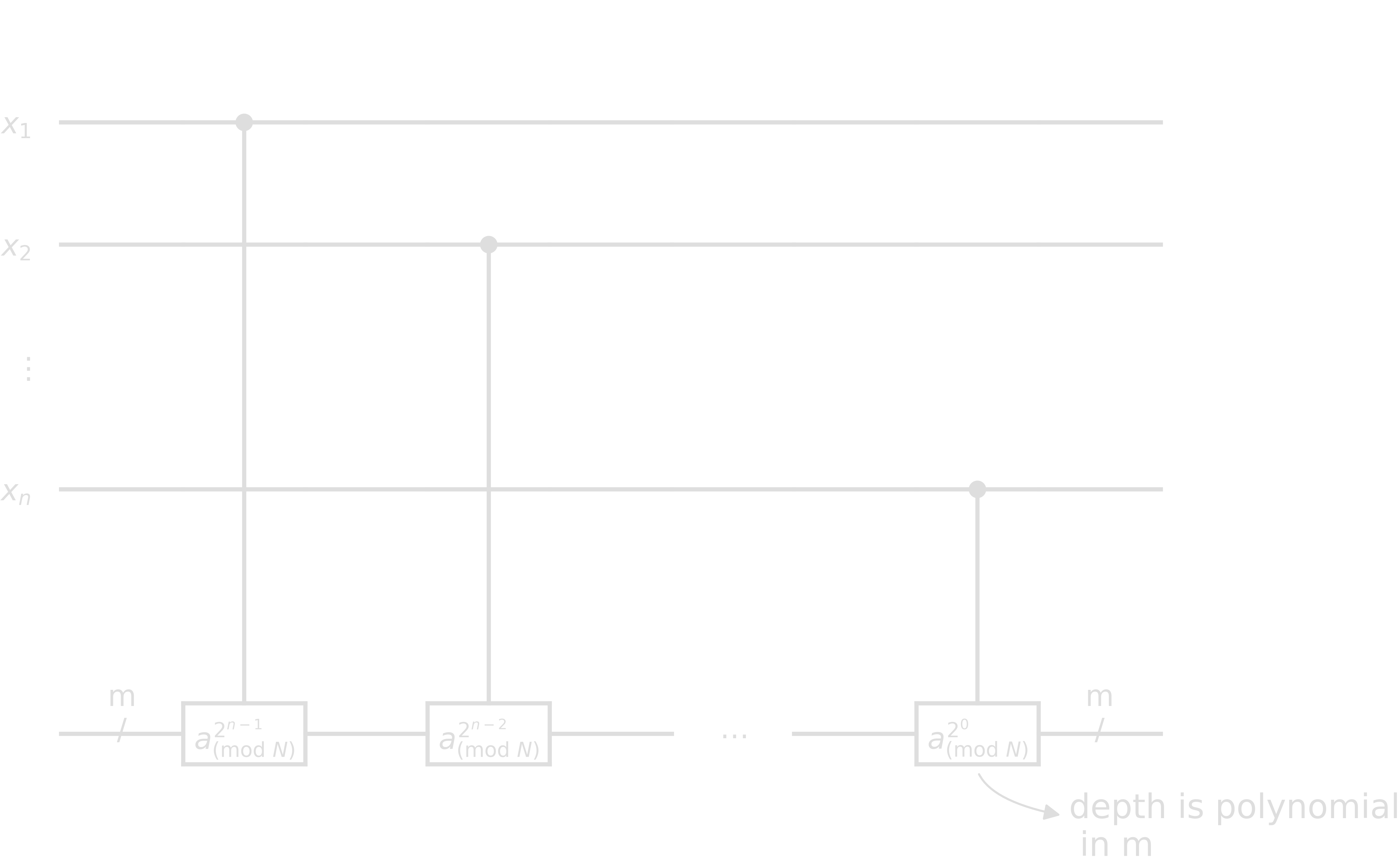
How to implement \(U_{f_{a N}}\)? Recall \(f_{a N}(x) \equiv a^x\ (\mathrm{mod}\ N)\) and
\[\begin{align} x =\ &\left[x_1\ x_2\ x_3\ \cdots\ x_n\right] = 2^{n-1}x_1 + 2^{n-2}x_2 + \cdots + 2^0x_n\\ f_{a N}(x) \equiv\ &a^x\ (\mathrm{mod}\ N)\\ =\ &a^{2^{n-1}x_1 + 2^{n-2}x_2 + \cdots + 2^0x_n}\ (\mathrm{mod}\ N)\\ =\ &a^{2^{n-1}x_1}a^{2^{n-2}x_2} \cdots a^{2^0x_n}\ (\mathrm{mod}\ N) \end{align}\]The circuit component is similar to QPE:
Quantum Error Correction
Superconducting qubits don’t work exactly as they should. Each gate is slightly imperfect, and influenced by (small) external forces. This is also true for spin qubits, topological qubits, photonic qubits, etc.
However, algorithms like Grover’s or Shor’s assume that qubits are perfect, so-called logical qubits, and imperfect qubits might cause these protocols to fail.
Many physical qubits can be used to create a logical qubit with quantum error correction. Examples of this are repetition code, surface code, with techniques like syndrome measurements, decoding, and logical operations.
Quantum error correction works analoguously to a simple situation: you are talking on the phone and need to answer a question with “yes” or “no”. There are two key points to consider: How likely is it that you will be misheard? This is given by the probability \(p\) that “no” sounds like “yes”, etc. And how much do you care about being misunderstood? This can be described by a maximum acceptable error probability \(P_a\). Usually \(p « P_a\), so there is no need to worry, but for important queries (life-or-death situations for instance) we cannot rely on probabilities and need to make sure.
The repetition code encoding supposes that repeated measurements are taken. With a lot of “no’s”, even with a few random “yes’s”, it’s obvious we mean “no”. With this encoding of our message, it has become tolerant to small faults. The receiver will have to decode the message. A sensible option is majority voting. A misunderstanding only happens when the majority of qubits are flipped. For \(d\) repetitions
\begin{equation} P = \sum_{n=0}^{d/2}\cvec{d \ n}p^{n}(1-p)^{d-n} \sim \left(\frac{p}{1-p}\right)^{d/2} \end{equation}
P decays with \(d\) exponentially, so with enough repetitions, we can make \(P\) as small as needed.
The basic features of any protocol for quantum error correction usually consist of:
- Input: some information to protect
- Encoding: transform the information to make it easier to protect
- Errors: Random pertubations and noise of the encoded message
- Decoding: trying to deduce the input from the perturbed message
For computations, errors can be introduced whenever an operation is performed. These errors need to be corrected as they are introduced, by constantly decoding and re-encoding. These schemes work great for bits, but for qubits decoding would require a measurement, and that destroys the state.
Break
Quantum error correction is a tricky subject, still very actively researched. Continuing on this path would make this post (if it isn’t already) waaayyy to long.
So, I’ll work on a second Part of this post where I dive into this subject more, and also show how to actually run code on a quantum computer using IBM’s qiskit module.
Also, if you’re interested in the graphics used in this post, have a look at the python scripts written by yours truly: