Deep-learning in visibility space
Why act in visibility space?
The sampling problem
Van Cittert-Zernike: \(\mathcal{V}(u,v) = \mathcal{F}\{A(l,m)\,I(l,m)\}\)
- Correlating at baselines → \((u,v)\) sample of Fourier attenuated sky
More \((u,v)\) samples → better \(\hat{I}\)
- Finite set of samples: image reconstruction is ill-posed
Every method closes the gap with a prior
- e.g. CLEAN assumes the sky is composed of point sources
- Problematic for faint, extended, complex structures
Our goal
- Generate missing visibility samples using DL "at acquisition time"
- Denoising and super-resolving the reconstructed image downstream
- Learning the prior instead of asserting it
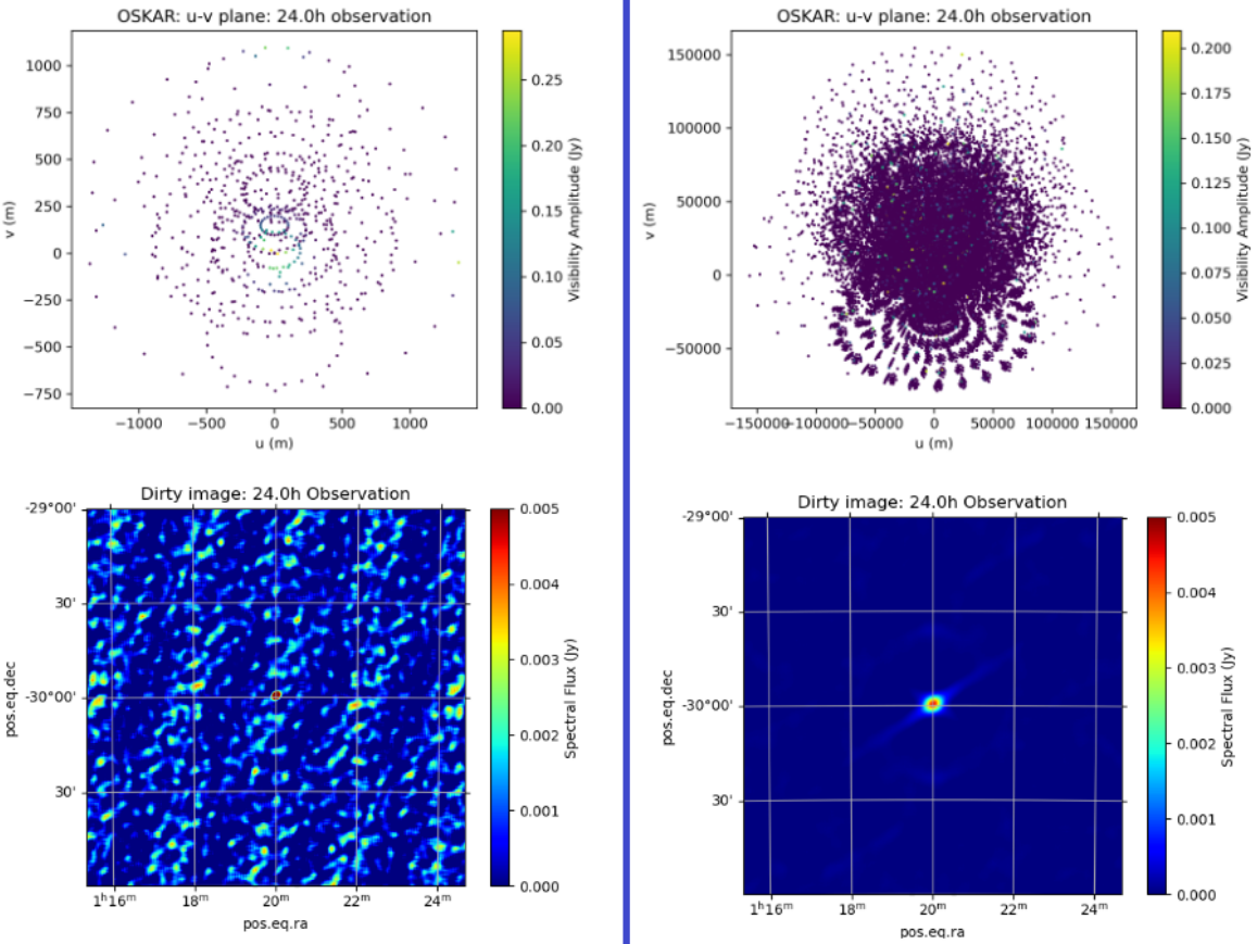
Figure 1: OSKAR, 24 h observation of the same sky. Left: SKA-Mid-AA1, 36 baselines. Right: AA4, 19,503 baselines. Top: \((u,v)\) coverage; bottom: the resulting dirty image.
Previous work
radionets
(Schmidt+22, Fröse+26) — the only close precedent:
- sampled cells in, complete \((u,v)\) plane out
- but one aggregated 2-D plane per observation — no time axis
- trained on a single array (VLBA — 10 antennas, 45 baselines)
- Low number of baselines
- time axis collapsed — one plane in, one plane out
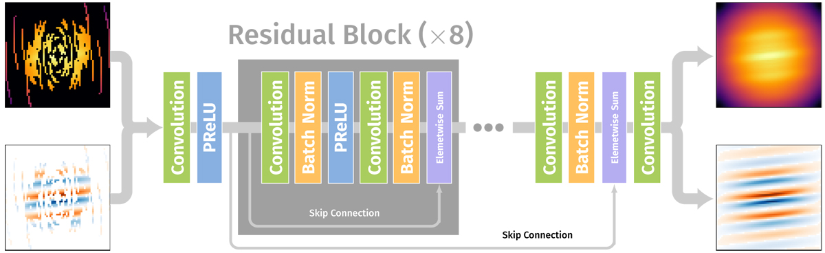
radionets approach: masked amplitude (top) and phase (bottom) of one finished \((u,v)\) plane in → dense amplitude and phase out, then an inverse FT to the image. 8 residual blocks, super-resolution CNN.
MSc thesis by Essahaty
(Thamena Essahaty, ZHAW × VUW Wellington NZ, 2026)
"Inferring Interference: Deep Learning for Radio Telescope Data Enhancement"
Supervised by Philipp Denzel (ZHAW) and Bing Xue (VUW).
Visibilities are large
Visibility tensor
One visibility tensor — SKA-Low:
\[V \in \mathbb{C}^{\,T \times F \times B \times P}\]
- T timesteps — @ 1s integrations (3600 for 1h)
- F frequency channels — \(O(10^2\) – \(10^5)\)
- B baselines — \(\frac{N(N-1)}{2}\) cross-correlations of N stations/dishes
- P polarisations, Stokes I, Q, U, and V
At complex64, scaling the baseline axis only ($T$=3600, $F$=64, $P$=4; window = 16 timesteps, stride 8 → 449 windows):
| stage | stations | baselines | file | window | timestep |
|---|---|---|---|---|---|
| AA2 | 64 | 2,016 | 13.8 GiB | 63 MiB | 3.94 MiB |
| AA∗ | 307 | 46,971 | 323 GiB | 1.43 GiB | 91.7 MiB |
| AA4 | 512 | 130,816 | 898 GiB | 3.99 GiB | 256 MiB |
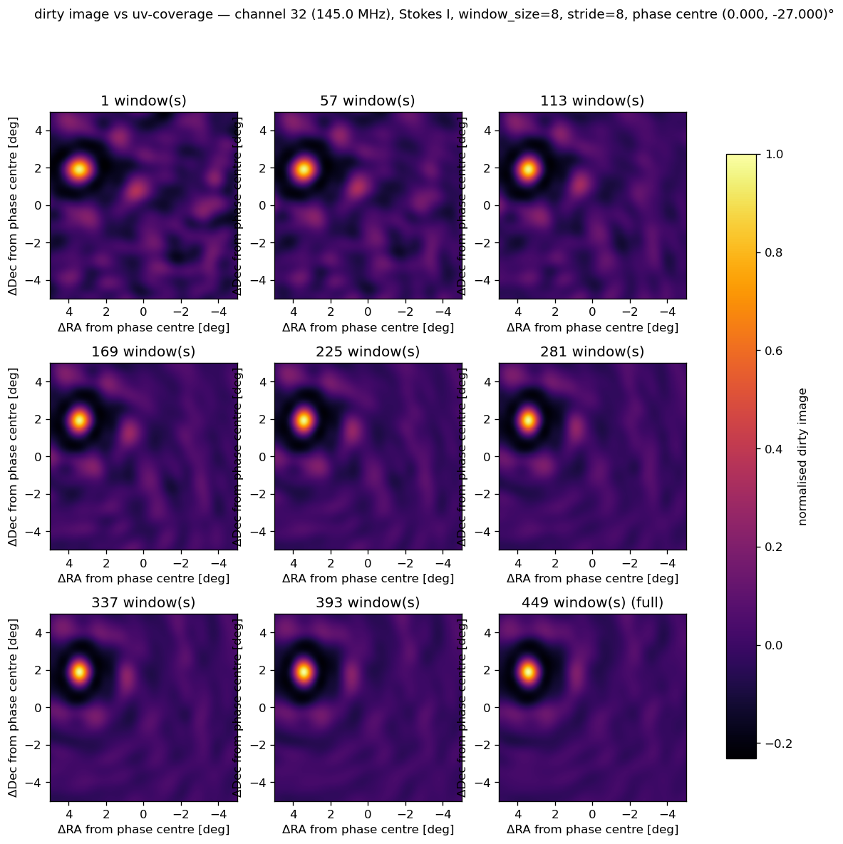
An SKA-Low AA2 simulation, 1 → 449 windows (2h): the sidelobes fall away as the Earth turns.
Basic SKA-Low AA2 GLEAM-like simulations
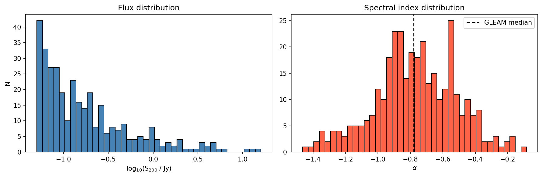
Figure 2: Synthetic catalogue: GLEAM-like flux and spectral-index distributions.
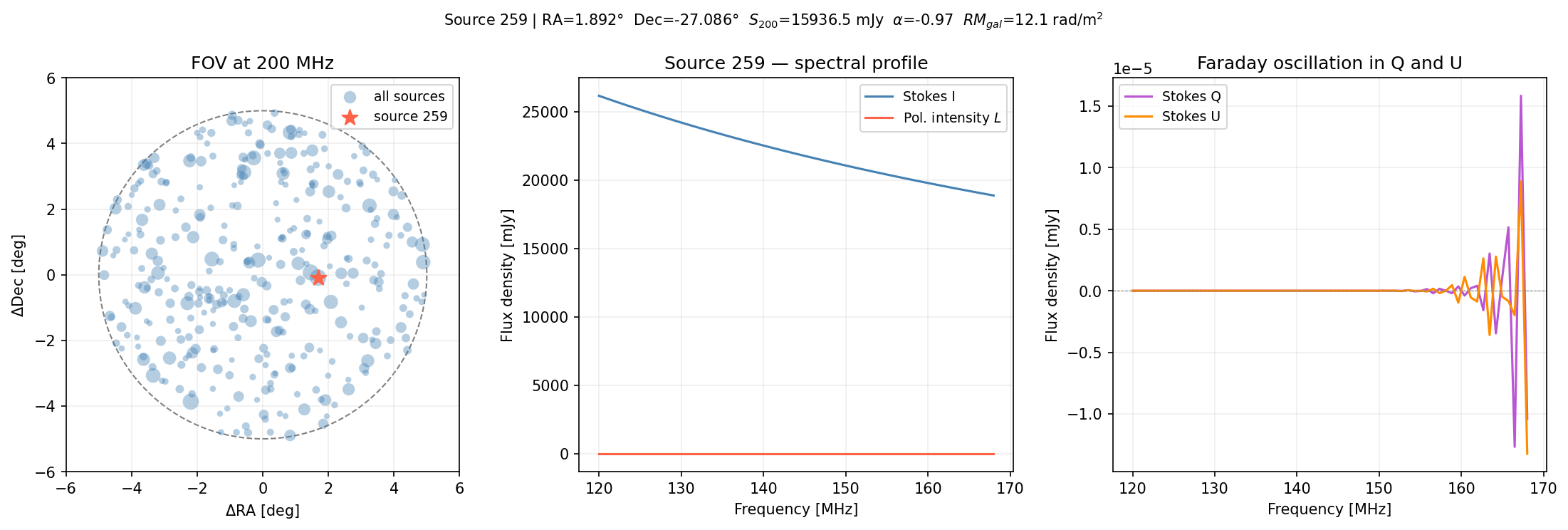
Figure 3: One realisation — 5° field at 200 MHz, per-source spectral profile, and the Faraday-rotated Q/U.
Polarization model
Simple model (intrinsic + galactic components) \[ P(\lambda^2) = p_0\times I\times\exp{\left( 2i (\chi_0 + \phi_\text{RM}\lambda^2) \right)} \times \mathcal{D}(\lambda^2) \]
where
- \(\phi_0\): intrinsic fractional polarization
- \(\chi_0\): intrinsic polarization angle
- \(\phi_\text{RM} = \text{RM}_\text{src} + \text{RM}_\text{gal}\): rotation measure
The galactic term, we fetch from Hutschenreuter+20 measurements - \(\mathcal{D}(\lambda^2)\): depolarization function
The Q and U terms are the real and imaginary parts of \(P(\lambda^2)\). The V term is in almost all cases 0.
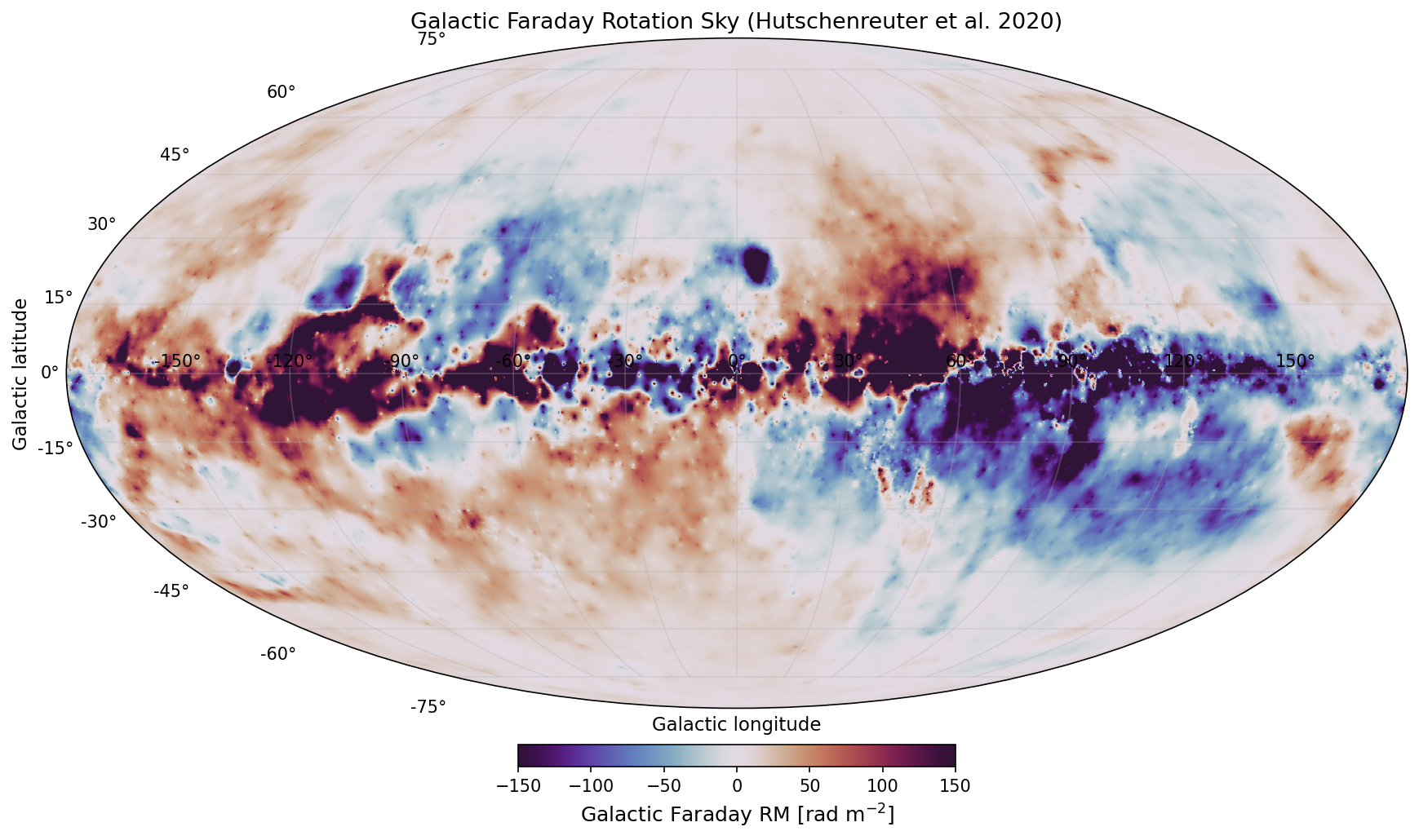
Figure 4: Galactic Faraday Rotation by Hutschenreuter+20.
A metric gap
200 simulations, centred sources, 50 epochs
| Model | PSNR (F) | PSNR (I) | MSSIM (I) |
|---|---|---|---|
| 3D patch ViT | 9.09 | 26.8 | 0.180 |
| 3D slice ViT | 25.2 | 31.5 | 0.530 |
| 3D U-Net | 27.4 | 32.4 | 0.683 |
1000 simulations, offset sources, 150 epochs
| Model | PSNR (F) | PSNR (I) | MSSIM (I) |
|---|---|---|---|
| 3D patch ViT | 6.87 | 23.6 | 0.120 |
| 3D slice ViT | 29.5 | 35.7 | 0.680 |
| 3D U-Net | 29.1 | 33.7 | 0.640 |
The U-Net won every metric while reconstructing almost nothing.
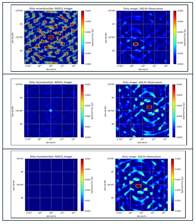
Reconstruction (left) vs. truth (right): patch ViT, slice ViT, U-Net.
Inductive bias must match the physics
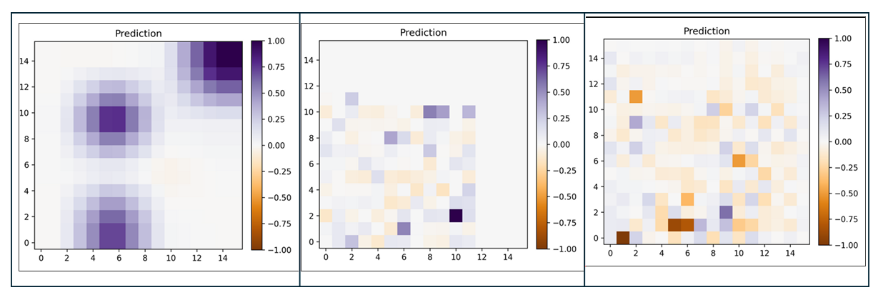
Predicted centre slices in the u-v plane. Left: patch ViT. Centre: slice ViT. Right: U-Net.
- Patch tokenisation assumes neighbouring pixels form a coherent spatial neighbourhood. In the Fourier domain adjacent frequels need not be adjacent baselines — so it hallucinated smooth, image-like blobs
- Convolutions assume locality and smoothness — also wrong for globally-coupled visibility data
- Slice tokenisation — one u-v slice per token, attention across time — matches the real structure, and wins once trivial solutions stop being rewarded
Representations are important: learning latents
Latent compression (200 epochs)
| Model / condition | PSNR (I) | MSSIM (I) |
|---|---|---|
| AE (f16) | 20.3 | 0.00 |
| AE (f16) + amplitude/phase | 24.4 | 0.08 |
| AE (f8) | 34.7 | 0.77 |
| AE (f8) + amplitude/phase | 41.9 | 0.92 |
- The latent respects the spatial-frequency coordinates better, and produces realistic emission
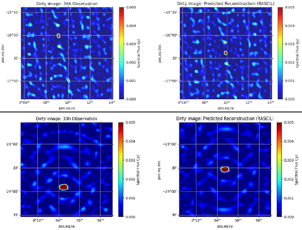
Latent forecasting still has problems — the learning objective splits the visibility into amplitude and phase, where amplitudes are prioritized without intervention. Phase contains positional information.
Compression — measured, axis by axis
- Time — Chebyshev, our best axis
- Frequency — compression ×2 but larger residual
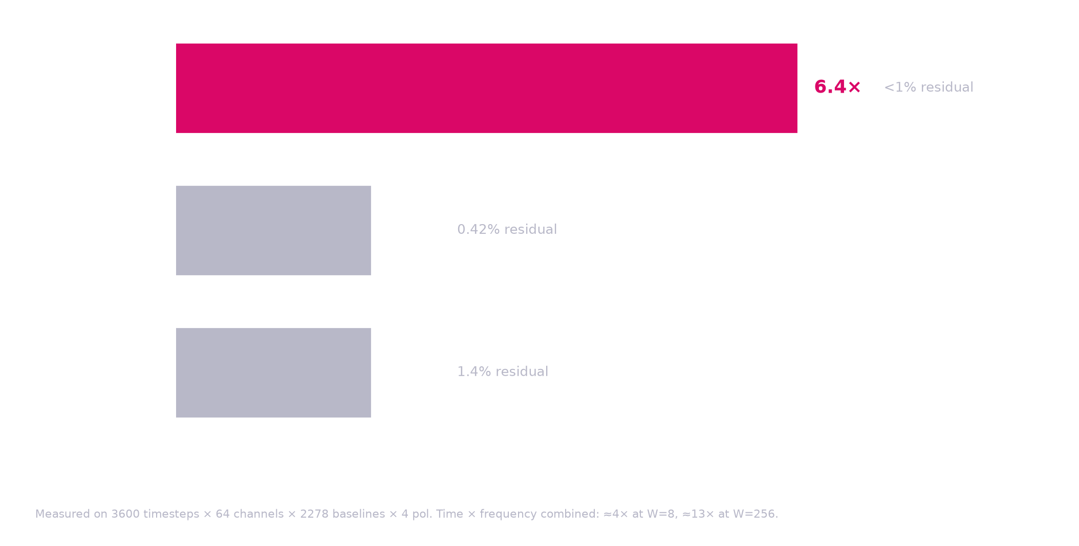
Time \(\times\) frequency: $≈$*13×* at $W$=256. The baseline axis gives nothing.
Deep compression
Deep Compression Autoencoder
(MIT Han Lab, arXiv:2410.10733) — the encoder behind NVIDIA's SANA:
- spatial compression 32×, 64×, 128×, where an SD-VAE stalls at 8×
dc-ae-f32c32: \(512\times512 \rightarrow 16\times16\times32\)- Residual autoencoding — learn residuals on space-to-channel transformed features
- Decoupled high-resolution adaptation — a three-phase training schedule
- 19.1× inference and 17.9× training speed-up on ImageNet-512, at better FID than SD-VAE-f8
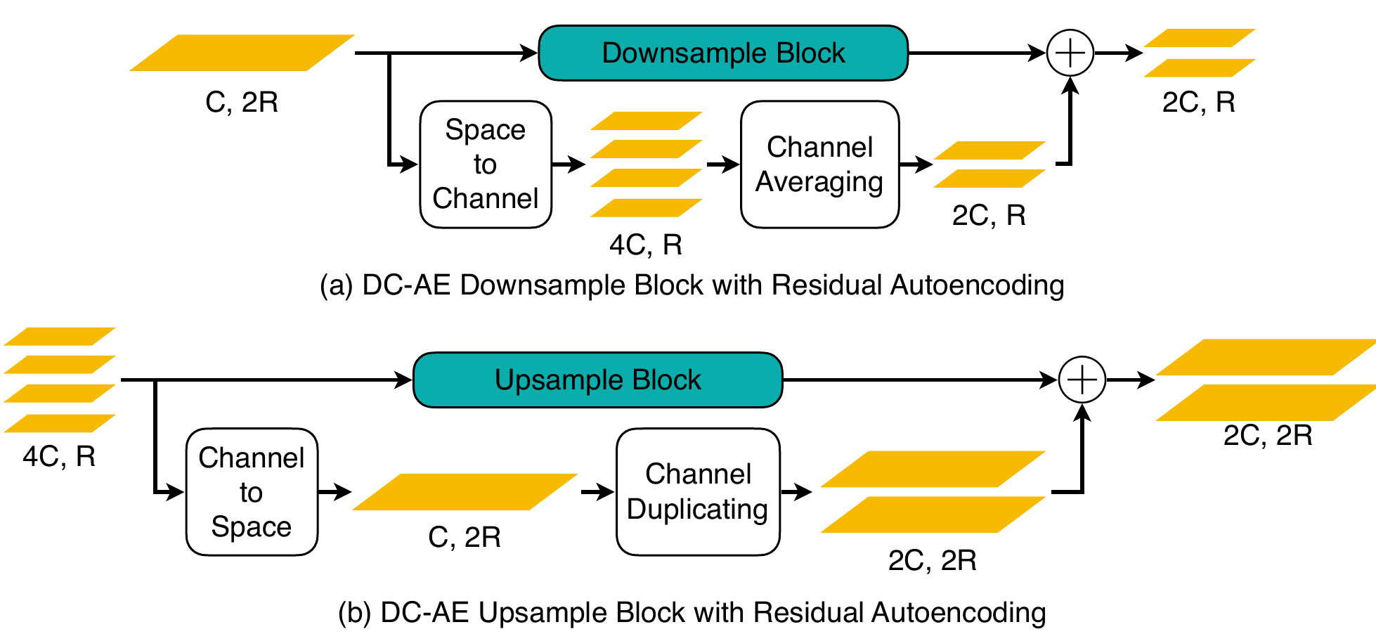
Residual autoencoding (Chen+25, Fig. 4). A non-parametric space-to-channel shortcut is added around every down- and upsample block, so the learned module only has to fit the residual: \(H\times W\times C \rightarrow \frac{H}{2}\times\frac{W}{2}\times 4C\), channel-averaged back to \(2C\). Nothing is discarded — resolution is traded for channels.
That shortcut is what makes 32–128× compression trainable at all.